BULLKpy - TCGA RNAseq data#
@mmm, January 23, 2026
2. Load original data into AnnData and BULLKpy object
3. Quality control and Preprocessing
4. PCA and Bidimensional Representation
5. Clustering and groups
6. Genes and Gene Signatures
7. Data Exploration
8. Associations & Correlations
9. Markers and Differential Expression
10. Pathway and Gene Enrichment Analysis
11. Metaprograms and Tumor Heterogeneity
12. Additional Plots
13. Utilities
1. Imports and settings#
1.1. Modules and Settings#
import os
import re
import numpy as np
import pandas as pd
import matplotlib as mpl
import matplotlib.pyplot as plt
import seaborn as sns

from datetime import datetime

import anndata as ad
import bullkpy as bk

import gseapy as gspy
from gseapy import Msigdb
from gseapy import gseaplot
from gseapy import enrichment_map
import sys
sys.version
print("Python:", sys.version, "Numpy:", np.__version__, "Pandas:", pd.__version__, "Matplotlib:", mpl.__version__, "Seaborn:", sns.__version__,
      "AnnData:", ad.__version__, "GSEApy:", gspy.__version__)
Python: 3.10.10 | packaged by conda-forge | (main, Mar 24 2023, 20:12:31) [Clang 14.0.6 ] Numpy: 1.23.5 Pandas: 2.3.3 Matplotlib: 3.8.0 Seaborn: 0.11.2 AnnData: 0.10.3 GSEApy: 1.1.0
bk.settings.verbosity = 3
bk.settings.plot_theme = "paper"      # "default" | "paper" | "talk"
bk.settings.plot_palette = "Set1"
bk.settings.plot_fontsize = 10        # optional
bk.settings.plot_dpi = 200
bk.settings.save_dpi = 300

# every plot calls set_style() internally, or you can call once:
bk.pl.set_style()
pal = sns.color_palette("husl", n_colors=35)       # palette for large categories
bk.settings.set_palette_for("Project_ID", where="obs", palette="husl")

import warnings
warnings.filterwarnings("ignore", category=FutureWarning, module="lifelines")
Change to paths with your files:
TCGA = "/Users/mmalumbres/Desktop/BioDATA/TCGA/"
DESKTOP = "/Users/mmalumbres/Desktop/"
2. Load data into AnnData and BULLKpy object#
Find details and additional parameters for all functions in:
https://bullkpy.readthedocs.io/en/latest/api/index.html
2.1. Load expression data#
TCGA data is available here:
https://portal.gdc.cancer.gov/
https://xenabrowser.net/datapages/
'GDC Pan-Cancer (PANCAN)/RNAseq/GDC-PANCAN.htseq_counts.tsv'
adata = bk.io.read_counts(TCGA + 'GDC Pan-Cancer (PANCAN)/RNAseq/GDC-PANCAN.htseq_counts.tsv', sep='\t',
                  orientation='genes_by_samples',
                  #dtype='int64'
                 )
adata
AnnData object with n_obs × n_vars = 11057 × 60488
Check Genes#
adata.var
| Ensembl_ID |
|---|
| ENSG00000000003.13 |
| ENSG00000000005.5 |
| ENSG00000000419.11 |
| ENSG00000000457.12 |
| ENSG00000000460.15 |
| ... |
| __no_feature |
| __ambiguous |
| __too_low_aQual |
| __not_aligned |
| __alignment_not_unique |
60488 rows × 0 columns
If you need to change .e.g from Ensembl IDs to gene symbols:#
download conversion table from biomart
change Ensembl IDs with gene symbols in adata.var_names
mask = adata.var_names.astype(str).str.startswith("ENS")
adata = adata[:, mask].copy()
adata.var
| Ensembl_ID |
|---|
| ENSG00000000003.13 |
| ENSG00000000005.5 |
| ENSG00000000419.11 |
| ENSG00000000457.12 |
| ENSG00000000460.15 |
| ... |
| ENSGR0000275287.3 |
| ENSGR0000276543.3 |
| ENSGR0000277120.3 |
| ENSGR0000280767.1 |
| ENSGR0000281849.1 |
60483 rows × 0 columns
adata.var_names = adata.var_names.str.split(".", n=1).str[0]
adata.var
| Ensembl_ID |
|---|
| ENSG00000000003 |
| ENSG00000000005 |
| ENSG00000000419 |
| ENSG00000000457 |
| ENSG00000000460 |
| ... |
| ENSGR0000275287 |
| ENSGR0000276543 |
| ENSGR0000277120 |
| ENSGR0000280767 |
| ENSGR0000281849 |
60483 rows × 0 columns
biomart_file = "/Users/mmalumbres/Desktop/BioDATA/Ensembl biomart/251224_biomart_export_gene_names.tsv"
gene_names = pd.read_csv(biomart_file, sep="\t")
gene_names.drop_duplicates(subset="Gene stable ID", keep="first", inplace=True)
gene_names = gene_names.set_index("Gene stable ID")
gene_names.head(3)
| Gene stable ID version | Transcript stable ID | Transcript stable ID version | Chromosome/scaffold name | Gene start (bp) | Gene end (bp) | Strand | Gene name | Source of gene name | Transcript name | Source of transcript name | Gene type | Gene Synonym | HGNC symbol | HGNC ID | |
|---|---|---|---|---|---|---|---|---|---|---|---|---|---|---|---|
| Gene stable ID | |||||||||||||||
| ENSG00000210049 | ENSG00000210049.1 | ENST00000387314 | ENST00000387314.1 | MT | 577 | 647 | 1 | MT-TF | HGNC Symbol | MT-TF-201 | Transcript name | Mt_tRNA | MTTF | MT-TF | HGNC:7481 |
| ENSG00000211459 | ENSG00000211459.2 | ENST00000389680 | ENST00000389680.2 | MT | 648 | 1601 | 1 | MT-RNR1 | HGNC Symbol | MT-RNR1-201 | Transcript name | Mt_rRNA | 12S | MT-RNR1 | HGNC:7470 |
| ENSG00000210077 | ENSG00000210077.1 | ENST00000387342 | ENST00000387342.1 | MT | 1602 | 1670 | 1 | MT-TV | HGNC Symbol | MT-TV-201 | Transcript name | Mt_tRNA | MTTV | MT-TV | HGNC:7500 |
var_genes = adata.var
var_genes = var_genes.merge(gene_names, how="left", left_index=True, right_index=True)
var_genes = var_genes.set_index("Gene name")
adata.var = var_genes
adata.var.head(3)
| Gene stable ID version | Transcript stable ID | Transcript stable ID version | Chromosome/scaffold name | Gene start (bp) | Gene end (bp) | Strand | Source of gene name | Transcript name | Source of transcript name | Gene type | Gene Synonym | HGNC symbol | HGNC ID | |
|---|---|---|---|---|---|---|---|---|---|---|---|---|---|---|
| Gene name | ||||||||||||||
| TSPAN6 | ENSG00000000003.17 | ENST00000373020 | ENST00000373020.9 | X | 100627108.0 | 100639991.0 | -1.0 | HGNC Symbol | TSPAN6-201 | Transcript name | protein_coding | T245 | TSPAN6 | HGNC:11858 |
| TNMD | ENSG00000000005.6 | ENST00000373031 | ENST00000373031.5 | X | 100584936.0 | 100599885.0 | 1.0 | HGNC Symbol | TNMD-201 | Transcript name | protein_coding | BRICD4 | TNMD | HGNC:17757 |
| DPM1 | ENSG00000000419.15 | ENST00000466152 | ENST00000466152.5 | 20 | 50934852.0 | 50959140.0 | -1.0 | HGNC Symbol | DPM1-205 | Transcript name | protein_coding | CDGIE | DPM1 | HGNC:3005 |
adata
AnnData object with n_obs × n_vars = 11057 × 60483
    var: 'Gene stable ID version', 'Transcript stable ID', 'Transcript stable ID version', 'Chromosome/scaffold name', 'Gene start (bp)', 'Gene end (bp)', 'Strand', 'Source of gene name', 'Transcript name', 'Source of transcript name', 'Gene type', 'Gene Synonym', 'HGNC symbol', 'HGNC ID'
Check Observations (Samples)#
Check samples or metadata (if any)
adata.obs
| TCGA-OR-A5JP-01A |
|---|
| TCGA-OR-A5JG-01A |
| TCGA-OR-A5K1-01A |
| TCGA-OR-A5JR-01A |
| TCGA-OR-A5KU-01A |
| ... |
| TCGA-WC-A87T-01A |
| TCGA-WC-AA9A-01A |
| TCGA-V4-A9EA-01A |
| TCGA-RZ-AB0B-01A |
| TCGA-V4-A9F8-01A |
11057 rows × 0 columns
Check expresion data
adata.X
array([[10,  2, 11, ...,  0,  0,  0],
       [10,  4, 11, ...,  0,  0,  0],
       [10,  1, 11, ...,  0,  0,  0],
       ...,
       [ 9,  0,  6, ...,  0,  0,  0],
       [ 9,  0, 10, ...,  0,  0,  0],
       [ 8,  0,  7, ...,  0,  0,  0]])
You can also use pandas or other python tools to read external data (counts, cpm, log-data etc.).
See “Other tools” section at the end of the notebook.
2.2. Load metadata#
Metadata store information relative to observations (Samples); e.g. tumor type; age of the patients, tumor purity, immune infiltration, survival, etc.
Edit all your available data in an external table (excel, csv, tsv etc.)
The “index_col” has be be identical to the listing of adata.obs above.
phenotype = '/GDC Pan-Cancer (PANCAN)/phenotype/GDC-PANCAN.TCGA_phenotype.tsv'
all_metadata = "260127_TCGA_metadata.tsv"
# Option 1 for easy metadata tables
adata = bk.add_metadata(adata,
                        TCGA + all_metadata,
                        low_memory=False,
                        sep="\t",
                        index_col="sample",)
adata.obs.head(3)
| Sample_ID | Patient_ID | Project_ID | gender | race | ajcc_pathologic_tumor_stage | clinical_stage | histological_type | histological_grade | initial_pathologic_dx_year | ... | SLIT2_mut | MYC_mut | MYCL_mut | MYCN_mut | SOX2_mut | ASCL1_mut | NEUROD1_mut | POU2F3_mut | YAP1_mut | NE25_score | |
|---|---|---|---|---|---|---|---|---|---|---|---|---|---|---|---|---|---|---|---|---|---|
| TCGA-OR-A5JP-01A | TCGA-OR-A5JP-01 | TCGA-OR-A5JP | ACC | MALE | WHITE | Stage II | NaN | Adrenocortical carcinoma- Usual Type | NaN | 2012.0 | ... | 0.0 | 0.0 | 0.0 | 0.0 | 0.0 | 0.0 | 0.0 | 0.0 | 0.0 | NaN |
| TCGA-OR-A5JG-01A | TCGA-OR-A5JG-01 | TCGA-OR-A5JG | ACC | MALE | WHITE | Stage IV | NaN | Adrenocortical carcinoma- Usual Type | NaN | 2008.0 | ... | 0.0 | 0.0 | 0.0 | 0.0 | 0.0 | 0.0 | 0.0 | 0.0 | 0.0 | NaN |
| TCGA-OR-A5K1-01A | TCGA-OR-A5K1-01 | TCGA-OR-A5K1 | ACC | MALE | WHITE | Stage II | NaN | Adrenocortical carcinoma- Usual Type | NaN | 2006.0 | ... | 0.0 | 0.0 | 0.0 | 0.0 | 0.0 | 0.0 | 0.0 | 0.0 | 0.0 | NaN |
3 rows × 1116 columns
adata
AnnData object with n_obs × n_vars = 11057 × 60483
    obs: 'Sample_ID', 'Patient_ID', 'Project_ID', 'gender', 'race', 'ajcc_pathologic_tumor_stage', 'clinical_stage', 'histological_type', 'histological_grade', 'initial_pathologic_dx_year', 'menopause_status', 'birth_days_to', 'vital_status', 'tumor_status', 'last_contact_days_to', 'death_days_to', 'cause_of_death', 'new_tumor_event_type', 'new_tumor_event_site', 'new_tumor_event_site_other', 'new_tumor_event_dx_days_to', 'treatment_outcome_first_course', 'margin_status', 'OS', 'OS.time', 'DSS', 'DSS.time', 'DFI', 'DFI.time', 'PFI', 'PFI.time', 'Redaction', 'Subtype_mRNA', 'Subtype_DNAmeth', 'Subtype_protein', 'Subtype_miRNA', 'Subtype_CNA', 'Subtype_Integrative', 'Subtype_other', 'Subtype_Selected', 'sample_type_id', 'sample_type', '_primary_disease', 'Subtype_Immune_Model_Based', 'ICS5_score', 'LIexpression_score', 'Chemokine12_score', 'NHI_5gene_score', 'CD68', 'CD8A', 'PD1_data', 'PDL1_data', 'PD1_PDL1_score', 'CTLA4_data', 'Bcell_mg_IGJ', 'Bcell_receptors_score', 'STAT1_score', 'CSF1_response', 'TcClassII_score', 'IL12_score_21050467', 'IL4_score_21050467', 'IL2_score_21050467', 'IL13_score_21050467', 'IFNG_score_21050467', 'TGFB_score_21050467', 'TREM1_data', 'DAP12_data', 'Tcell_receptors_score', 'IL8_21978456', 'IFN_21978456', 'MHC1_21978456', 'MHC2_21978456', 'Bcell_21978456', 'Tcell_21978456', 'CD103pos_mean_25446897', 'CD103neg_mean_25446897', 'IgG_19272155', 'Interferon_19272155', 'LCK_19272155', 'MHC.I_19272155', 'MHC.II_19272155', 'STAT1_19272155', 'Troester_WoundSig_19887484', 'MDACC.FNA.1_20805453', 'IGG_Cluster_21214954', 'Minterferon_Cluster_21214954', 'Immune_cell_Cluster_21214954', 'MCD3_CD8_21214954', 'Interferon_Cluster_21214954', 'B_cell_PCA_16704732', 'CD8_PCA_16704732', 'GRANS_PCA_16704732', 'LYMPHS_PCA_16704732', 'T_cell_PCA_16704732', 'TGFB_PCA_17349583', 'Rotterdam_ERneg_PCA_15721472', 'HER2_Immune_PCA_18006808', 'IR7_score', 'Buck14_score', 'TAMsurr_score', 'Immune_NSCLC_score', 'Module3_IFN_score', 'Module4_TcellBcell_score', 'Module5_TcellBcell_score', 'Module11_Prolif_score', 'GP11_Immune_IFN', 'GP2_ImmuneTcellBcell_score', 'CD8_CD68_ratio', 'TAMsurr_TcClassII_ratio', 'CHANG_CORE_SERUM_RESPONSE_UP', 'CSR_Activated_15701700', 'CD103pos_CD103neg_ratio_25446897', 'ai1', 'lst1', 'hrd-loh', 'HRD', 'GP1_Proliferation/DNA_repair', 'GP2_Immune-Tcell/Bcell', 'GP3_Tumor_suppressing_miRNA_targets', 'GP4_MES/ECM', 'GP5_MYC_targets/TERT', 'GP6_Squamous_differentiation/development', 'GP7_Estrogen_signaling', 'GP8_FOXO/stemness', 'GP9_Cell-cell_adhesion', 'GP10_Fatty_acid_oxidation', 'GP11_Immune-IFN_GP12_Hypoxia/glycolosis', 'GP13_Neural_signailng', 'GP14_Plasma_membrane_cell-cell_signaling', 'GP15_EGF_signailng', 'GP16_Protein_kinase_signailng_(MAPKs)', 'GP17_Basal_signaling', 'GP18_Vesicle/EPR_membrane_coat', 'GP19_1Q_amplicon', 'GP20_TAL1-Leukemia/erythropoiesis', 'GP21_Anti-apoptosis/DNA_stability', 'GP22_16Q22-24_amplicon', 'AKT_PATHWAY', 'ALK_PATHWAY', 'BRCA_ATR_PATHWAY', 'CASPASE_CASCADE_(APOPTOSIS)', 'CTLA4_PATHWAY', 'HDAC_TARGETS_DN', 'HER2_AMPLIFIED', 'IGF1R_PATHWAY', 'MTOR_PATHWAY', 'MYC_amplified', 'PD1_SIGNALING', 'PI3K_CASCADE', 'PTEN_PATHWAY', 'RAS_PATHWAY', 'RB_PATHWAY', 'RESPONSE_TO_ANDROGEN', 'RETINOL_METABOLISM', 'VEGF_PATHWAY', 'Genome_doublings', 'AS', 'Aneu', 'AS_amp', 'AS_del', 'WAS', 'WAneu', 'WAS_amp', 'WAS_del', 'Leuk', 'Stroma', 'Stroma_notLeukocyte', 'Stroma_notLeukocyte_Floor', 'SilentMutationspeMb', 'Non-silentMutationsperMb', '1p', '1q', '2p', '2q', '3p', '3q', '4p', '4q', '5p', '5q', '6p', '6q', '7p', '7q', '8p', '8q', '9p', '9q', '10p', '10q', '11p', '11q', '12p', '12q', '13q', '14q', '15q', '16p', '16q', '17p', '17q', '18p', '18q', '19p', '19q', '20p', '20q', '21q', '22q', 'chr01', 'chr02', 'chr03', 'chr04', 'chr05', 'chr06', 'chr07', 'chr08', 'chr09', 'chr10', 'chr11', 'chr12', 'chr13', 'chr14', 'chr15', 'chr16', 'chr17', 'chr18', 'chr19', 'chr20', 'chr21', 'chr22', 'sample.1', 'program', 'project_id_TCGA', 'Age at Diagnosis in Years', 'Gender', '_PATIENT', 'demographic.age_at_index', 'demographic.created_datetime', 'demographic.days_to_birth', 'demographic.days_to_death', 'demographic.demographic_id', 'demographic.ethnicity', 'demographic.gender', 'demographic.race', 'demographic.state', 'demographic.submitter_id', 'demographic.updated_datetime', 'demographic.vital_status', 'demographic.year_of_birth', 'demographic.year_of_death', 'diagnoses.age_at_diagnosis', 'diagnoses.classification_of_tumor', 'diagnoses.created_datetime', 'diagnoses.days_to_diagnosis', 'diagnoses.days_to_last_follow_up', 'diagnoses.diagnosis_id', 'diagnoses.icd_10_code', 'diagnoses.last_known_disease_status', 'diagnoses.morphology', 'diagnoses.primary_diagnosis', 'diagnoses.prior_malignancy', 'diagnoses.prior_treatment', 'diagnoses.progression_or_recurrence', 'diagnoses.site_of_resection_or_biopsy', 'diagnoses.state', 'diagnoses.submitter_id', 'diagnoses.synchronous_malignancy', 'diagnoses.tissue_or_organ_of_origin', 'diagnoses.tumor_grade', 'diagnoses.tumor_stage', 'diagnoses.updated_datetime', 'diagnoses.year_of_diagnosis', 'exposures.alcohol_history', 'exposures.bmi', 'exposures.cigarettes_per_day', 'exposures.created_datetime', 'exposures.exposure_id', 'exposures.height', 'exposures.pack_years_smoked', 'exposures.state', 'exposures.submitter_id', 'exposures.updated_datetime', 'exposures.weight', 'exposures.years_smoked', 'id', 'project.name', 'project.project_id', 'tissue_source_site.name', 'samples.is_ffpe', 'samples.sample_id', 'samples.sample_type', 'samples.sample_type_id', 'samples.tissue_type', 'array', 'call status', 'purity', 'ploidy', 'Genome doublings', 'Coverage for 80% power', 'Cancer DNA fraction', 'Subclonal genome fraction', 'solution', 'Unnamed: 0', 'bcr_patient_barcode', 'type', 'PFI.1', 'PFI.time.1', 'PFI.2', 'PFI.time.2', 'PFS', 'PFS.time', 'DSS_cr', 'DSS.time.cr', 'DFI.cr', 'DFI.time.cr', 'PFI.cr', 'PFI.time.cr', 'PFI.1.cr', 'PFI.time.1.cr', 'PFI.2.cr', 'PFI.time.2.cr', 'bcr_patient_uuid', 'acronym', 'gender_y', 'days_to_birth', 'days_to_death', 'days_to_last_followup', 'days_to_initial_pathologic_diagnosis', 'icd_10', 'tissue_retrospective_collection_indicator', 'icd_o_3_histology', 'tissue_prospective_collection_indicator', 'history_of_neoadjuvant_treatment', 'icd_o_3_site', 'tumor_tissue_site', 'new_tumor_event_after_initial_treatment', 'radiation_therapy', 'project_code', 'prior_dx', 'disease_code', 'ethnicity', 'informed_consent_verified', 'person_neoplasm_cancer_status', 'patient_id_short', 'year_of_initial_pathologic_diagnosis', 'histological_type_y', 'tissue_source_site', 'form_completion_date', 'pathologic_T', 'pathologic_M', 'clinical_M', 'pathologic_N', 'system_version', 'pathologic_stage', 'stage_other', 'clinical_T', 'clinical_N', 'extranodal_involvement', 'postoperative_rx_tx', 'primary_therapy_outcome_success', 'lymph_node_examined_count', 'primary_lymph_node_presentation_assessment', 'initial_pathologic_diagnosis_method', 'number_of_lymphnodes_positive_by_he', 'eastern_cancer_oncology_group', 'anatomic_neoplasm_subdivision', 'residual_tumor', 'histological_type_other', 'init_pathology_dx_method_other', 'karnofsky_performance_score', 'neoplasm_histologic_grade', 'height', 'weight', 'history_of_radiation_metastatic_site', 'days_to_patient_progression_free', 'days_to_first_response', 'days_to_first_partial_response', 'days_to_first_complete_response', 'days_to_tumor_progression', 'er_estimated_duration_response', 'er_disease_extent_prior_er_treatment', 'er_solid_tumor_response_documented_type', 'er_solid_tumor_response_documented_type_other', 'er_response_type', 'history_of_radiation_primary_site', 'history_prior_surgery_type', 'patient_progression_status', 'history_prior_surgery_type_other', 'history_prior_surgery_indicator', 'field', 'molecular_abnormality_results_other', 'molecular_abnormality_results', 'number_of_lymphnodes_positive_by_ihc', 'tobacco_smoking_history', 'number_pack_years_smoked', 'stopped_smoking_year', 'performance_status_scale_timing', 'laterality', 'targeted_molecular_therapy', 'year_of_tobacco_smoking_onset', 'anatomic_neoplasm_subdivision_other', 'patient_death_reason', 'tumor_tissue_site_other', 'age_began_smoking_in_years', 'kras_gene_analysis_performed', 'kras_mutation_found', 'death_cause_text', 'lactate_dehydrogenase_result', 'days_to_sample_procurement', 'hbv_test', 'on_haart_therapy_at_cancer_diagnosis', 'hcv_test', 'prior_aids_conditions', 'on_haart_therapy_prior_to_cancer_diagnosis', 'kshv_hhv8_test', 'days_to_hiv_diagnosis', 'hiv_status', 'hiv_rna_load_at_diagnosis', 'cdc_hiv_risk_group', 'history_of_other_malignancy', 'history_immunosuppresive_dx', 'nadir_cd4_counts', 'history_relevant_infectious_dx_other', 'history_relevant_infectious_dx', 'cd4_counts_at_diagnosis', 'history_immunological_disease_other', 'hpv_test', 'history_immunosuppressive_dx_other', 'history_immunological_disease', 'lost_follow_up', 'venous_invasion', 'lymphatic_invasion', 'perineural_invasion_present', 'her2_erbb_method_calculation_method_text', 'her2_immunohistochemistry_level_result', 'breast_carcinoma_immunohistochemistry_pos_cell_score', 'distant_metastasis_present_ind2', 'her2_erbb_pos_finding_fluorescence_in_situ_hybridization_calculation_method_text', 'breast_carcinoma_immunohistochemistry_progesterone_receptor_pos_finding_scale', 'breast_carcinoma_primary_surgical_procedure_name', 'er_level_cell_percentage_category', 'breast_carcinoma_progesterone_receptor_status', 'breast_carcinoma_surgical_procedure_name', 'breast_neoplasm_other_surgical_procedure_descriptive_text', 'er_detection_method_text', 'pos_finding_progesterone_receptor_other_measurement_scale_text', 'her2_erbb_pos_finding_cell_percent_category', 'her2_and_centromere_17_positive_finding_other_measurement_scale_text', 'pos_finding_metastatic_breast_carcinoma_estrogen_receptor_other_measuremenet_scale_text', 'metastatic_breast_carcinoma_progesterone_receptor_level_cell_percent_category', 'metastatic_breast_carcinoma_pos_finding_progesterone_receptor_other_measure_scale_text', 'fluorescence_in_situ_hybridization_diagnostic_procedure_chromosome_17_signal_result_range', 'first_recurrent_non_nodal_metastatic_anatomic_site_descriptive_text', 'first_nonlymph_node_metastasis_anatomic_site', 'immunohistochemistry_positive_cell_score', 'axillary_lymph_node_stage_method_type', 'axillary_lymph_node_stage_other_method_descriptive_text', 'metastatic_breast_carcinoma_progesterone_receptor_status', 'metastatic_breast_carcinoma_immunohistochemistry_pr_pos_cell_score', 'metastatic_breast_carcinoma_immunohistochemistry_er_pos_cell_score', 'metastatic_breast_carcinoma_lab_proc_her2_neu_immunohistochemistry_receptor_status', 'metastatic_breast_carcinoma_her2_neu_chromosone_17_signal_ratio_value', 'surgical_procedure_purpose_other_text', 'metastatic_breast_carcinoma_her2_erbb_pos_finding_fluorescence_in_situ_hybridization_calculation_method_text', 'metastatic_breast_carcinoma_her2_erbb_pos_finding_cell_percent_category', 'breast_cancer_surgery_margin_status', 'metastatic_breast_carcinoma_her2_erbb_method_calculation_method_text', 'breast_carcinoma_estrogen_receptor_status', 'her2_neu_and_centromere_17_copy_number_analysis_input_total_number_count', 'pgr_detection_method_text', 'pos_finding_her2_erbb2_other_measurement_scale_text', 'breast_carcinoma_immunohistochemistry_er_pos_finding_scale', 'positive_finding_estrogen_receptor_other_measurement_scale_text', 'metastatic_breast_carcinoma_erbb2_immunohistochemistry_level_result', 'metastatic_breast_carcinoma_pos_finding_other_scale_measurement_text', 'her2_neu_chromosone_17_signal_ratio_value', 'cytokeratin_immunohistochemistry_staining_method_micrometastasis_indicator', 'metastatic_breast_carcinoma_estrogen_receptor_detection_method_text', 'metastatic_breast_carcinoma_lab_proc_her2_neu_in_situ_hybridization_outcome_type', 'metastatic_breast_carcinoma_pos_finding_her2_erbb2_other_measure_scale_text', 'lab_proc_her2_neu_immunohistochemistry_receptor_status', 'progesterone_receptor_level_cell_percent_category', 'metastatic_breast_carcinoma_estrogen_receptor_level_cell_percent_category', 'metastatic_breast_carcinoma_estrogen_receptor_status', 'lab_procedure_her2_neu_in_situ_hybrid_outcome_type', 'her2_neu_breast_carcinoma_copy_analysis_input_total_number', 'metastatic_breast_carcinoma_fluorescence_in_situ_hybridization_diagnostic_proc_centromere_17_signal_result_range', 'her2_neu_and_centromere_17_copy_number_metastatic_breast_carcinoma_analysis_input_total_number_count', 'her2_neu_metastatic_breast_carcinoma_copy_analysis_input_total_number', 'metastatic_breast_carcinoma_progesterone_receptor_detection_method_text', 'additional_pharmaceutical_therapy', 'additional_radiation_therapy', 'lymphovascular_invasion_present', 'pos_lymph_node_location_other', 'pos_lymph_node_location', 'location_in_lung_parenchyma', 'pulmonary_function_test_performed', 'pre_bronchodilator_fev1_fvc_percent', 'kras_mutation_result', 'post_bronchodilator_fev1_percent', 'pre_bronchodilator_fev1_percent', 'dlco_predictive_percent', 'egfr_mutation_performed', 'diagnosis', 'eml4_alk_translocation_result', 'egfr_mutation_result', 'post_bronchodilator_fev1_fvc_percent', 'eml4_alk_translocation_performed', 'eml4_alk_translocation_method', 'days_to_new_tumor_event_after_initial_treatment', 'hemoglobin_result', 'serum_calcium_result', 'platelet_qualitative_result', 'number_of_lymphnodes_positive', 'erythrocyte_sedimentation_rate_result', 'white_cell_count_result', 'malignant_neoplasm_metastatic_involvement_site', 'other_metastatic_involvement_anatomic_site', 'birth_control_pill_history_usage_category', 'alcohol_history_documented', 'frequency_of_alcohol_consumption', 'source_of_patient_death_reason', 'days_to_diagnostic_mri_performed', 'days_to_diagnostic_computed_tomography_performed', 'amount_of_alcohol_consumption_per_day', 'family_history_of_cancer', 'loss_expression_of_mismatch_repair_proteins_by_ihc_result', 'preoperative_pretreatment_cea_level', 'microsatellite_instability', 'number_of_loci_tested', 'history_of_colon_polyps', 'number_of_first_degree_relatives_with_cancer_diagnosis', 'number_of_abnormal_loci', 'circumferential_resection_margin', 'non_nodal_tumor_deposits', 'braf_gene_analysis_result', 'colon_polyps_present', 'kras_mutation_codon', 'braf_gene_analysis_performed', 'synchronous_colon_cancer_present', 'loss_expression_of_mismatch_repair_proteins_by_ihc', 'barretts_esophagus', 'city_of_procurement', 'reflux_history', 'country_of_procurement', 'antireflux_treatment_type', 'h_pylori_infection', 'hypertension', 'horm_ther', 'pln_pos_ihc', 'surgical_approach', 'pregnancies', 'diabetes', 'peritoneal_wash', 'pct_tumor_invasion', 'prior_tamoxifen_administered_usage_category', 'colorectal_cancer', 'total_aor-lnp', 'pln_pos_light_micro', 'total_pelv_lnp', 'total_pelv_lnr', 'aln_pos_light_micro', 'aln_pos_ihc', 'total_aor_lnr', 'post_surgical_procedure_assessment_thyroid_gland_carcinoma_status', 'metastatic_neoplasm_confirmed_diagnosis_method_text', 'metastatic_neoplasm_confirmed_diagnosis_method_name', 'prior_glioma', 'tumor_residual_disease', 'jewish_origin', 'distant_metastasis_anatomic_site', 'new_neoplasm_event_type', 'lymphnode_dissection_method_left', 'lymphnode_neck_dissection', 'egfr_amplication_status', 'hpv_status_by_ish_testing', 'presence_of_pathological_nodal_extracapsular_spread', 'p53_gene_analysis', 'hpv_status_by_p16_testing', 'lymphnode_dissection_method_right', 'eml4_alk_translocation_identified', 'egfr_mutation_identified', 'supratentorial_localization', 'mold_or_dust_allergy_history', 'motor_movement_changes', 'inherited_genetic_syndrome_found', 'seizure_history', 'asthma_history', 'first_diagnosis_age_asth_ecz_hay_fev_mold_dust', 'first_diagnosis_age_of_food_allergy', 'ldh1_mutation_found', 'tumor_location', 'ldh1_mutation_test_method', 'animal_insect_allergy_types', 'first_presenting_symptom', 'animal_insect_allergy_history', 'first_presenting_symptom_longest_duration', 'ldh1_mutation_tested', 'visual_changes', 'first_diagnosis_age_of_animal_insect_allergy', 'history_ionizing_rt_to_head', 'sensory_changes', 'food_allergy_history', 'mental_status_changes', 'hay_fever_history', 'preoperative_corticosteroids', 'preoperative_antiseizure_meds', 'family_history_of_primary_brain_tumor', 'inherited_genetic_syndrome_result', 'days_to_initial_score_performance_status_scale', 'food_allergy_types', 'headache_history', 'eczema_history', 'other_genotyping_outcome_lab_results_text', 'extrathyroid_carcinoma_present_extension_status', 'i_131_first_administered_dose', 'i_131_subsequent_administered_dose', 'i_131_total_administered_dose', 'primary_neoplasm_focus_type', 'i_131_total_administered_preparation_technique', 'person_lifetime_risk_radiation_exposure_indicator', 'ret_ptc_rearrangement_genotyping_outcome_lab_results_text', 'genotyping_results_gene_mutation_not_reported_reason', 'neoplasm_depth', 'genotype_analysis_performed_indicator', 'ras_family_gene_genotyping_outcome_lab_results_text', 'neoplasm_length', 'neoplasm_width', 'radiosensitizing_agent_administered_indicator', 'braf_gene_genotyping_outcome_lab_results_text', 'lymph_node_preoperative_scan_indicator', 'radiation_therapy_administered_preparation_technique_text', 'lymph_node_preoperative_assessment_diagnostic_imaging_type', 'patient_personal_medical_history_thyroid_gland_disorder_name', 'first_degree_relative_history_thyroid_gland_carcinoma_diagnosis_relationship_type', 'radiation_therapy_administered_dose_text', 'patient_personal_medical_history_thyroid_other_specify_text', 'primary_thyroid_gland_neoplasm_location_anatomic_site', 'lymphnodes_examined', 'zone_of_origin', 'days_to_bone_scan_performed', 'diagnostic_mri_performed', 'diagnostic_mri_result', 'psa_value', 'days_to_first_biochemical_recurrence', 'secondary_pattern', 'primary_pattern', 'diagnostic_ct_abd_pelvis_result', 'bone_scan_results', 'biochemical_recurrence', 'tumor_level', 'gleason_score', 'number_of_lymphnodes_examined', 'days_to_psa', 'tertiary_pattern', 'diagnostic_ct_abd_pelvis_performed', 'family_medical_history_relative_family_member_relationship_type', 'tumor_type', 'primary_tumor_multiple_present_ind', 'prior_systemic_therapy_type', 'melanoma_clark_level_value', 'melanoma_origin_skin_anatomic_site', 'malignant_neoplasm_mitotic_count_rate', 'breslow_depth_value', 'tumor_tissue_site.1', 'melanoma_ulceration_indicator', 'primary_neoplasm_melanoma_dx', 'new_tumor_dx_prior_submitted_specimen_dx', 'primary_anatomic_site_count', 'interferon_90_day_prior_excision_admin_indicator', 'primary_melanoma_at_diagnosis_count', 'days_to_submitted_specimen_dx', 'antireflux_treatment', 'number_of_relatives_with_stomach_cancer', 'family_history_of_stomach_cancer', 'state_province_country_of_procurement', 'specimen_collection_method_name', 'child_pugh_classification_grade', 'hist_of_non_mibc', 'occupation_primary_job', 'person_concomitant_prostate_carcinoma_occurrence_indicator', 'person_concomitant_prostate_carcinoma_pathologic_t_stage', 'cancer_diagnosis_cancer_type_icd9_text_name', 'non_mibc_tx', 'bladder_carcinoma_extracapsular_extension_status', 'chemical_exposure_text', 'resp_maint_from_bcg_admin_month_dur', 'maint_therapy_course_complete', 'induction_course_complete', 'person_occupation_years_number', 'person_primary_industry_text', 'disease_extracapsular_extension_ind-3', 'complete_response_observed', 'diagnosis_subtype', 'diagnosis_age', 'mibc_90day_post_resection_bcg', 'person_occupation_description_text', 'surgical_procedure_name_other_specify_text', 'relative_family_cancer_history_ind_3', 'vascular_tumor_cell_invasion_type', 'viral_hepatitis_serology', 'liver_fibrosis_ishak_score_category', 'ablation_embolization_tx_adjuvant', 'laboratory_procedure_prothrombin_time_result_value', 'laboratory_procedure_creatinine_result_lower_limit_of_normal_value', 'laboratory_procedure_alpha_fetoprotein_outcome_value', 'laboratory_procedure_alpha_fetoprotein_outcome_upper_limit_of_normal_value', 'laboratory_procedure_alpha_fetoprotein_outcome_lower_limit_of_normal_value', 'laboratory_procedure_albumin_result_upper_limit_of_normal_value', 'laboratory_procedure_albumin_result_specified_value', 'laboratory_procedure_creatinine_result_upper_limit_of_normal_value', 'laboratory_prcoedure_platelet_result_upper_limit_of_normal_value', 'lab_procedure_platelet_result_specified_value', 'days_to_definitive_surgical_procedure_performed', 'hematology_serum_creatinine_laboratory_result_value_in_mg_dl', 'history_hepato_carcinoma_risk_factor', 'history_hepato_carcinoma_risk_factor_other', 'cancer_diagnosis_first_degree_relative_number', 'laboratory_prcoedure_platelet_result_lower_limit_of_normal_value', 'laboratory_procedure_international_normalization_ratio_result_lower_limit_of_normal_value', 'laboratory_procedure_albumin_result_lower_limit_of_normal_value', 'laboratory_procedure_total_bilirubin_result_specified_lower_limit_of_normal_value', 'laboratory_procedure_total_bilirubin_result_specified_upper_limit_of_normal_value', 'laboratory_procedure_total_bilirubin_result_upper_limit_normal_value', 'adjacent_hepatic_tissue_inflammation_extent_type', 'laboratory_procedure_international_normalization_ratio_result_upper_limit_of_normal_value', 'mitotic_count', 'oligonucleotide_primer_pair_laboratory_procedure_performed_name', 'radiation_type_notes', 'number_of_successful_pregnancies_which_resulted_in_at_least_1_live_birth', 'external_beam_radiation_therapy_administered_paraaortic_region_lymph_node_dose', 'concurrent_chemotherapy_dose', 'chemotherapy_regimen_type', 'chemotherapy_negation_radiation_therapy_concurrent_not_administered_reason', 'postoperative_rx_tx.1', 'dose_frequency_text', 'rt_pelvis_administered_total_dose', 'cervical_neoplasm_pathologic_margin_involved_type', 'cervical_neoplasm_pathologic_margin_involved_text', 'cervical_carcinoma_pelvic_extension_text', 'cervical_carcinoma_corpus_uteri_involvement_indicator', 'ectopic_pregnancy_count', 'rt_administered_type', 'oligonucleotide_primer_pair_laboratory_procedure_performed_text', 'other_chemotherapy_agent_administration_specify', 'radiation_therapy_not_administered_reason', 'patient_pregnancy_therapeutic_abortion_count', 'days_to_laboratory_procedure_tumor_marker_squamous_cell_carcinoma_antigen_result', 'days_to_performance_status_assessment', 'prescribed_dose_units', 'diagnostic_ct_result_outcome', 'patient_pregnancy_spontaneous_abortion_count', 'patient_pregnancy_count', 'fdg_or_ct_pet_performed_outcome', 'female_breast_feeding_or_pregnancy_status_indicator', 'standardized_uptake_value_cervix_uteri_assessment_measurement', 'pregnant_at_diagnosis', 'pregnancy_stillbirth_count', 'patient_history_immune_system_and_related_disorders_text', 'patient_history_immune_system_and_related_disorders_name', 'days_to_fdg_or_ct_pet_performed', 'diagnostic_mri_result_outcome', 'radiation_therapy.1', 'radiation_therapy_not_administered_specify', 'human_papillomavirus_laboratory_procedure_performed_name', 'chemotherapy_negation_radiation_therapy_concurrent_administered_text', 'lymph_node_location_positive_pathology_name', 'keratinizing_squamous_cell_carcinoma_present_indicator', 'laboratory_procedure_tumor_marker_squamous_cell_carcinoma_antigen_result_value', 'total_number_of_pregnancies', 'hysterectomy_Performed_Ind-3', 'hysterectomy_performed_text', 'human_papillomavirus_other_type_text', 'hysterectomy_performed_type', 'lymphovascular_invasion_indicator', 'brachytherapy_first_reference_point_administered_total_dose', 'brachytherapy_method_other_specify_text', 'lymph_node_location_positive_pathology_text', 'tumor_response_cdus_type', 'brachytherapy_method_type', 'agent_total_dose_count', 'live_birth_number', 'human_papillomavirus_laboratory_procedure_performed_text', 'human_papillomavirus_type', 'performance_status_assessment_timepoint_category_other_text', 'ct_scan', 'new_neoplasm_event_occurrence_anatomic_site', 'radiologic_tumor_width', 'contiguous_organ_resection_site', 'radiologic_tumor_depth', 'radiologic_tumor_burden', 'tumor_depth', 'pathologic_tumor_width', 'tumor_multifocal', 'other_contiguous_organ_resection_site', 'contiguous_organ_invaded', 'pathologic_tumor_length', 'pathologic_tumor_depth', 'pathologic_tumor_burden', 'radiologic_tumor_length', 'tumor_total_necrosis_percent', 'primary_tumor_lower_uterus_segment', 'days_to_well_differentiated_liposarcoma_resection', 'metastatic_site_at_diagnosis_other', 'metastatic_site_at_diagnosis', 'ss18_ssx_testing_method', 'ss18_ssx_fusion_status', 'specific_tumor_total_necrosis_percent', 'leiomyosarcoma_histologic_subtype', 'metastatic_neoplasm_confirmed', 'local_disease_recurrence', 'days_to_well_differentiated_liposarcoma_primary_dx', 'mpnst_neurofibromatosis', 'mpnst_exisiting_plexiform_neurofibroma', 'mpnst_nf1_genetic_testing', 'mpnst_specific_mutations', 'well_differentiated_liposarcoma_primary_dx', 'leiomyosarcoma_major_vessel_involvement', 'discontiguous_lesion_count', 'mpnst_neurofibromatosis_heredity', 'maximum_tumor_dimension', 'alcoholic_exposure_category', 'planned_surgery_status', 'esophageal_tumor_involvement_site', 'esophageal_tumor_cental_location', 'lymph_node_metastasis_radiographic_evidence', 'days_to_pancreatitis_onset', 'days_to_diabetes_onset', 'adenocarcinoma_invasion', 'surgery_performed_type', 'columnar_metaplasia_present', 'relative_cancer_type', 'amt_alcohol_consumption_per_day', 'columnar_mucosa_goblet_cell_present', 'history_of_chronic_pancreatitis', 'history_of_diabetes', 'goblet_cells_present', 'history_of_esophageal_cancer', 'histologic_grading_tier_category', 'columnar_mucosa_dysplasia', 'number_of_relatives_diagnosed', 'state_province_of_procurement', 'treatment_prior_to_surgery', 'initial_diagnosis_by', 'surgery_performed_type_other', 'country_of_birth', 'disease_detected_on_screening', 'history_pheo_or_para_include_benign', 'outside_adrenal', 'history_pheo_or_para_anatomic_site', 'family_member_relationship_type', 'post_op_ablation_embolization_tx', 'days_to_pre_orchi_serum_test', 'post_orchi_hcg', 'bilateral_diagnosis_timing_type', 'post_orchi_ldh', 'testis_tumor_microextent', 'undescended_testis_corrected', 'post_orchi_lh', 'post_orchi_lymph_node_dissection', 'post_orchi_testosterone', 'serum_markers', 'undescended_testis_corrected_age', 'undescended_testis_method_left', 'relation_testicular_cancer', 'postoperative_tx', 'testis_tumor_macroextent', 'synchronous_tumor_histology_pct', 'pre_orchi_afp', 'pre_orchi_hcg', 'pre_orchi_ldh', 'pre_orchi_lh', 'pre_orchi_testosterone', 'synchronous_tumor_histology_type', 'relative_family_cancer_hx_text', 'days_to_post_orchi_serum_test', 'undescended_testis_method_right', 'testis_tumor_macroextent_other', 'days_to_bilateral_tumor_dx', 'level_of_non_descent', 'post_orchi_afp', 'intratubular_germ_cell_neoplasm', 'igcccg_stage', 'history_of_undescended_testis', 'molecular_test_result', 'history_hypospadias', 'history_fertility', 'histological_percentage', 'first_treatment_success', 'family_history_testicular_cancer', 'family_history_other_cancer', 'masaoka_stage', 'history_myasthenia_gravis', 'section_myasthenia_gravis', 'new_neoplasm_occurrence_anatomic_site_text', 'percent_tumor_sarcomatoid', 'presence_of_sarcomatoid_features', 'tmem127', 'therapeutic_mitotane_lvl_recurrence', 'therapeutic_mitotane_lvl_macroscopic_residual', 'therapeutic_mitotane_levels_achieved', 'metastatic_neoplasm_initial_diagnosis_anatomic_site', 'mitoses_count', 'mitotane_therapy', 'mitotane_therapy_adjuvant_setting', 'mitotane_therapy_for_macroscopic_residual_disease', 'mitotic_rate', 'sinusoid_invasion', 'therapeutic_mitotane_lvl_progression', 'excess_adrenal_hormone_diagnosis_method_type', 'molecular_analysis_performed_indicator', 'excess_adrenal_hormone_history_type', 'necrosis', 'sdhd', 'sdhc', 'nuclear_grade_III_IV', 'sdhb', 'sdhaf2_sdh5', 'sdha', 'atypical_mitotic_figures', 'ct_scan_findings', 'ret', 'cytoplasm_presence_less_than_equal_25_percent', 'weiss_venous_invasion', 'weiss_score', 'vhl', 'invasion_of_tumor_capsule', 'diffuse_architecture', 'serum_mesothelin_lower_limit', 'asbestos_exposure_type', 'pleurodesis_performed_90_days', 'mesothelioma_detection_method', 'history_asbestos_exposure', 'pleurodesis_performed_prior', 'family_history_cancer_type', 'family_history_cancer_type_other', 'asbestos_exposure_age', 'serum_mesothelin_prior_tx', 'asbestos_exposure_years', 'serum_mesothelin_upper_limit', 'asbestos_exposure_source', 'suv_of_pleura_max', 'primary_occupation', 'primary_occupation_years_worked', 'primary_occupation_other', 'creatinine_norm_range_lower', 'creatinine_norm_range_upper', 'asbestos_exposure_age_last', 'creatinine_prior_tx', 'tumor_basal_diameter', 'tumor_basal_diameter_mx', 'metastatic_site', 'tumor_thickness', 'microvascular_density_mvd', 'tumor_shape_pathologic_clinical', 'tumor_infiltrating_lymphocytes', 'tumor_morphology_percentage', 'tumor_thickness_measurement', 'tumor_infiltrating_macrophages', 'pet_ct_standardized_values', 'eye_color', 'other_metastatic_site', 'extravascular_matrix_patterns', 'histological_type.1', 'extranocular_nodule_size', 'extrascleral_extension', 'gene_expression_profile', 'cytogenetic_abnormality', 'result_of_immunophenotypic_analysis', 'prior_immunosuppressive_therapy_other', 'prior_immunosuppressive_therapy_type', 'prior_infectious_disease', 'igk_genotype_results.1', 'immunophenotypic_analysis_method', 'igk_genotype_results', 'bone_marrow_biopsy_done', 'bone_marrow_involvement', 'bone_marrow_involvement.1', 'prior_infectious_disease_other', 'ebv_positive_malignant_cells_percent', 'b_lymphocyte_genotyping_method.1', 'prior_immunologic_disease_type', 'igh_genotype_results.1', 'b_lymphocyte_genotyping_method', 'prior_immunologic_disease_other', 'maximum_tumor_bulk_anatomic_location', 'immunophenotypic_analysis_results', 'maximum_tumor_bulk_anatomic_site', 'immunophenotypic_analysis_test', 'extranodal_sites_involvement_number', 'immunophenotypic_analysis_tested', 'ebv_status_malignant_cells_method', 'percent_ebv_positive_malignant_cells', 'tumor_resected_max_dimension', 'immunophenotypic_analysis_methodology', 'igh_genotype_results', 'ebv_diagnostic_methodology', 'follicular_component_percent', 'abnormality_tested_methodology', 'nodal_anatomic_site', 'histology_of_bone_marrow_sample', 'abnormality_tested_methodology.1', 'ldh_upper_limit', 'number_of_involved_extranodal_sites', 'extranodal_disease_involvement_site', 'ebv_antibody_status', 'extranodal_disease_involvement_site_other', 'genetic_abnormality_tested_other', 'genetic_abnormality_tested.1', 'genetic_abnormality_tested', 'genetic_abnormality_results_other', 'genetic_abnormality_results', 'percentage_of_follicular_component', 'pet_scan_results', 'other_genetic_abnormality_tested', 'epstein_barr_viral_status', 'lymph_node_involvement_site', 'mib1_positive_percentage_range', 'mib1_positive_percentage_range.1', 'genetic_abnormality_method_other', 'extranodal_involvment_site_other', 'ldh_lab_value', 'hiv_positive_status', 'ldh_level', 'ldh_norm_range_upper', 'abnormality_tested_results.1', 'abnormality_tested_results', 'genetic_abnormality_method', 'bone_marrow_sample_histology', 'albumin_result_upper_limit', 'vascular_tumor_cell_type', 'albumin_result_lower_limit', 'albumin_result_specified_value', 'platelet_result_upper_limit', 'intern_norm_ratio_upper_limit', 'cholangitis_tissue_evidence', 'relative_family_cancer_history', 'platelet_result_lower_limit', 'hist_hepato_carcinoma_risk', 'hist_hepato_carc_fact', 'cancer_first_degree_relative', 'creatinine_lower_level', 'prothrombin_time_result_value', 'ca_19_9_level_upper', 'ca_19_9_level_lower', 'ca_19_9_level', 'creatinine_upper_limit', 'surgical_procedure_name', 'creatinine_value_in_mg_dl', 'bilirubin_lower_limit', 'total_bilirubin_upper_limit', 'platelet_result_count', 'fibrosis_ishak_score', 'fetoprotein_outcome_value', 'fetoprotein_outcome_upper_limit', 'fetoprotein_outcome_lower_limit', 'inter_norm_ratio_lower_limit', 'family_cancer_type_txt', 'bilirubin_upper_limit', 'days_to_last_known_alive', 'Unnamed: 1061', 'Unnamed: 1062', 'n_genes_detected', 'leiden_0.2', 'leiden_0.4', 'leiden_0.6', 'leiden_0.8', 'leiden_1', 'leiden_1.2', 'leiden_1.5', 'leiden_2', 'leiden_2.2', 'kmeans_10', 'kmeans_15', 'kmeans_20', 'kmeans_25', 'kmeans_30', 'Proliferation_score', 'T_cell_score', 'Neuroendocrine_score', 'score_prolif', 'S_score', 'G2M_score', 'phase', 'TP53_mut', 'RB1_mut', 'KRAS_mut', 'EGFR_mut', 'KEAP1_mut', 'NFE2L2_mut', 'STK11_mut', 'PIK3CA_mut', 'SMARCA4_mut', 'BRAF_mut', 'PTEN_mut', 'CDKN2A_mut', 'CCND1_mut', 'NOTCH1_mut', 'CREBBP_mut', 'EP300_mut', 'KMT2D_mut', 'KMT2C_mut', 'NOTCH1.1_mut', 'NOTCH2_mut', 'NOTCH3_mut', 'SLIT2_mut', 'MYC_mut', 'MYCL_mut', 'MYCN_mut', 'SOX2_mut', 'ASCL1_mut', 'NEUROD1_mut', 'POU2F3_mut', 'YAP1_mut', 'NE25_score'
    var: 'Gene stable ID version', 'Transcript stable ID', 'Transcript stable ID version', 'Chromosome/scaffold name', 'Gene start (bp)', 'Gene end (bp)', 'Strand', 'Source of gene name', 'Transcript name', 'Source of transcript name', 'Gene type', 'Gene Synonym', 'HGNC symbol', 'HGNC ID'
2.3. Save AnnData object#
adata.write("../data/h5ad/260127_TCGA_example_in_BULLKpy.h5ad", compression="gzip")
If you find problems writing to .h5ad or with the format of the columns go to the last section (Other Tools) in this notebook
3. Quality Control and preprocessing#
If you are not sure about the format of the expression data:
# Integer (counts) or log transformed?
print("Are expression data integers: counts?")
X = adata.layers["counts"] if "counts" in adata.layers else adata.X
bk.pp._is_integerish(X)
Are expression data integers: counts?
True
# If counts, Save counts in a separata layer before normalization and log
### SKIP if data are already log-transformed
bk.pp.set_raw_counts(adata)      # layers["counts"]
3.1. Compute QC#
If counts:
bk.pp.qc_metrics(adata, layer="counts")
If log data:
bk.pp.qc_metrics(adata, layer="log1p_cpm", detection_threshold=0.1)
will compute only n_genes_detected and warn about skipping count-based metrics
adata.var.head(3)
| Gene stable ID version | Transcript stable ID | Transcript stable ID version | Chromosome/scaffold name | Gene start (bp) | Gene end (bp) | Strand | Source of gene name | Transcript name | Source of transcript name | Gene type | Gene Synonym | HGNC symbol | HGNC ID | |
|---|---|---|---|---|---|---|---|---|---|---|---|---|---|---|
| Gene name | ||||||||||||||
| TSPAN6 | ENSG00000000003.17 | ENST00000373020 | ENST00000373020.9 | X | 100627108.0 | 100639991.0 | -1.0 | HGNC Symbol | TSPAN6-201 | Transcript name | protein_coding | T245 | TSPAN6 | HGNC:11858 |
| TNMD | ENSG00000000005.6 | ENST00000373031 | ENST00000373031.5 | X | 100584936.0 | 100599885.0 | 1.0 | HGNC Symbol | TNMD-201 | Transcript name | protein_coding | BRICD4 | TNMD | HGNC:17757 |
| DPM1 | ENSG00000000419.15 | ENST00000466152 | ENST00000466152.5 | 20 | 50934852.0 | 50959140.0 | -1.0 | HGNC Symbol | DPM1-205 | Transcript name | protein_coding | CDGIE | DPM1 | HGNC:3005 |
bk.pp.qc_metrics(adata, layer="counts", detection_threshold=5,
                mt_prefix='MT-',
                )
# will compute only n_genes_detected and warn about skipping count-based metrics
3.2. Visual QC overview#
#If you only computed n_genes_detected
bk.pl.qc_metrics(
    adata,
    #color="n_genes_detected",
    #vars_to_plot=("n_genes_detected",)
    save=DESKTOP + "qc_metrics_example.png",
);
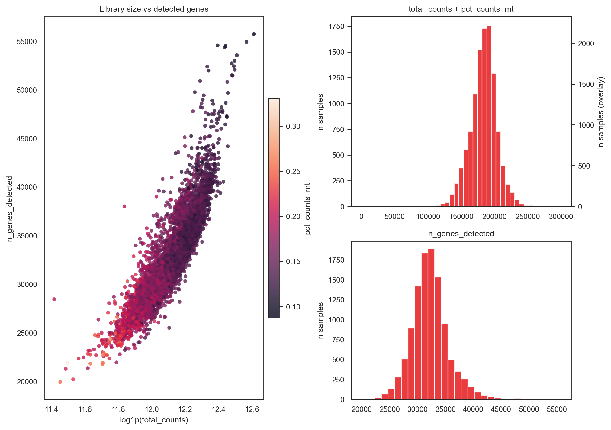
Filter out poor quality samples or genes#
adata.obs[["n_genes_detected"]].describe() #"total_counts", "pct_counts_mt"
| n_genes_detected | |
|---|---|
| count | 11057.000000 |
| mean | 32314.838473 |
| std | 3423.261879 |
| min | 19943.000000 |
| 25% | 30246.000000 |
| 50% | 32087.000000 |
| 75% | 33983.000000 |
| max | 55739.000000 |
Filter out poor samples or genes
If counts: use
layer="counts"If normalized,
use layer="cpm"If log-transformed, use
layer="log1p_cpm"
# keep genes expressed in a minumum of X samples and with expression above a thershol
adata = bk.pp.filter_genes(adata, layer="counts", min_samples=20, min_expr=10)
# keep samples with a minimum of genes detected and minimum expression per gene
adata = bk.pp.filter_samples(adata, layer="counts", min_genes=15000, expr_threshold_for_genes=10)
# 4) Recompute QC after gene filtering (optional but nice)
bk.pp.qc_metrics(adata, layer="counts", detection_threshold=10)
Normalize (skip is already normalized)#
bk.pp.normalize_cpm(adata) # layers["cpm"]
Log-transform (skip is already normalized and log-transformed)#
bk.pp.log1p(adata) # layers["log1p_cpm"]
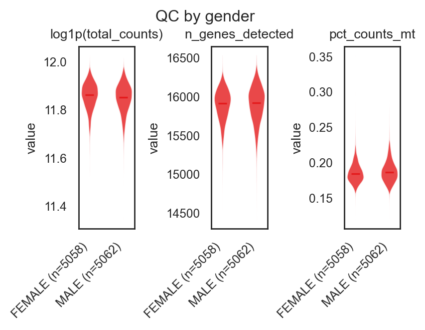
3.2. Visual QC overview#
bk.pl.qc_by_group(adata, groupby="gender",
                  keys=('total_counts', 'n_genes_detected', 'pct_counts_mt'),
                  figsize=(4,3),
                  save=DESKTOP + "qc_by_group_example.png",
                 )
(<Figure size 800x600 with 3 Axes>,
 array([<Axes: title={'center': 'log1p(total_counts)'}, ylabel='value'>,
        <Axes: title={'center': 'n_genes_detected'}, ylabel='value'>,
        <Axes: title={'center': 'pct_counts_mt'}, ylabel='value'>],
       dtype=object))
bk.pl.qc_pairplot(adata, keys=('total_counts', 'n_genes_detected', 'pct_counts_mt',),
                  save=DESKTOP + "qc_pairplot_example.png",
                  point_size=10,
                 )
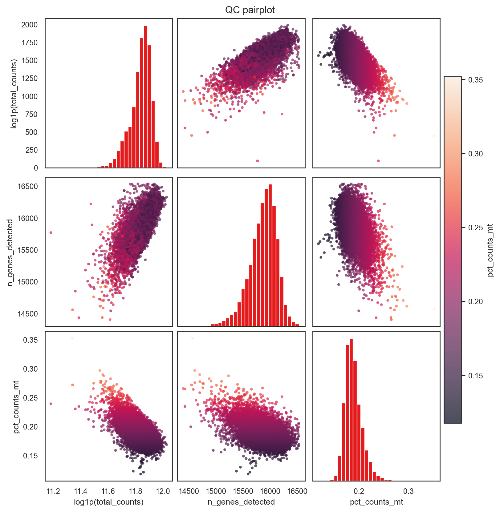
(<Figure size 1600x1600 with 10 Axes>,
 array([[<Axes: ylabel='log1p(total_counts)'>, <Axes: >, <Axes: >],
        [<Axes: ylabel='n_genes_detected'>, <Axes: >, <Axes: >],
        [<Axes: xlabel='log1p(total_counts)', ylabel='pct_counts_mt'>,
         <Axes: xlabel='n_genes_detected'>,
         <Axes: xlabel='pct_counts_mt'>]], dtype=object))
Store AnnData object with metrics
adata.write("../data/h5ad/260127_TCGA_example_in_BULLKpy.h5ad", compression="gzip")
4. PCA and bidimensional representation#
# Open .h5ad file if previously stored
adata = ad.read_h5ad("../data/h5ad/251226_BULLKpy_TCGA_RNAseq.h5ad")
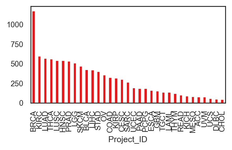
fig, ax = plt.subplots(figsize=(4,2), dpi=200)
adata.obs["Project_ID"].value_counts().plot(kind="bar")
<Axes: xlabel='Project_ID'>
4.1. Highly-variable genes & PCA#
bk.pp.highly_variable_genes(adata, layer="log1p_cpm", n_top_genes=2000)
adata.var["highly_variable"].sum()
2000
If you ever see HVGs dominated by: • mitochondrial genes • ribosomal genes
you may want to exclude them before HVG selection:
mask = ~adata.var_names.str.startswith(("MT-", "RPS", "RPL"))adata_hvg = adata[:, mask].copy()bk.pp.highly_variable_genes(adata_hvg, ...)
# Compute PCA
bk.tl.pca(adata, layer="log1p_cpm", n_comps=20,
         use_highly_variable=True,)                              # typically better to use only highly-variable genes
bk.pl.pca_scatter(adata, color="Project_ID", palette="tab20", figsize=(3,2.8), point_size=2,
                 save=DESKTOP + "pca_projectID.png")

# palette "tab20", "husl"...
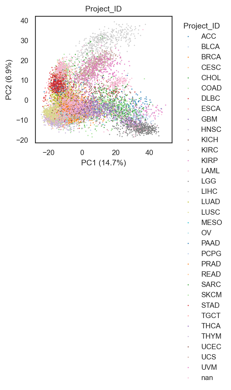
(<Figure size 600x560 with 1 Axes>,
 [<Axes: title={'center': 'Project_ID'}, xlabel='PC1 (14.7%)', ylabel='PC2 (6.9%)'>])
bk.pl.pca_scatter(adata, color="GFAP", layer="log1p_cpm", cmap="viridis", point_size=2, figsize=(3,2.5))
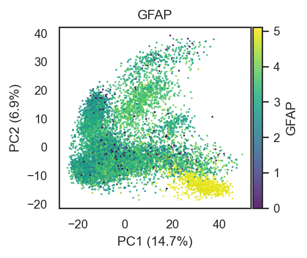
(<Figure size 600x500 with 2 Axes>,
 [<Axes: title={'center': 'GFAP'}, xlabel='PC1 (14.7%)', ylabel='PC2 (6.9%)'>])
bk.pl.pca_scatter(adata, color="histological_grade", point_size=2, figsize=(3.8,2.5))
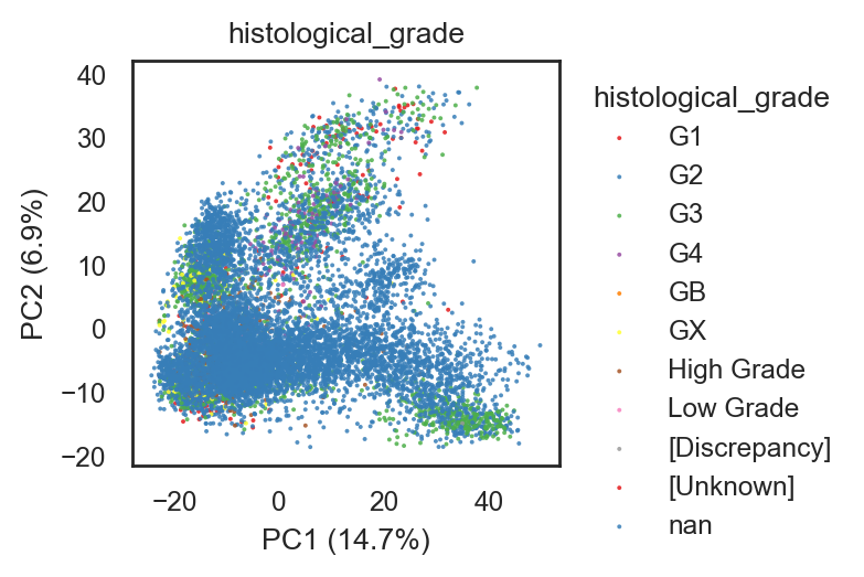
(<Figure size 760x500 with 1 Axes>,
 [<Axes: title={'center': 'histological_grade'}, xlabel='PC1 (14.7%)', ylabel='PC2 (6.9%)'>])
bk.pl.pca_scatter(adata, color="purity", point_size=2, figsize=(3,2.5), cmap="magma")
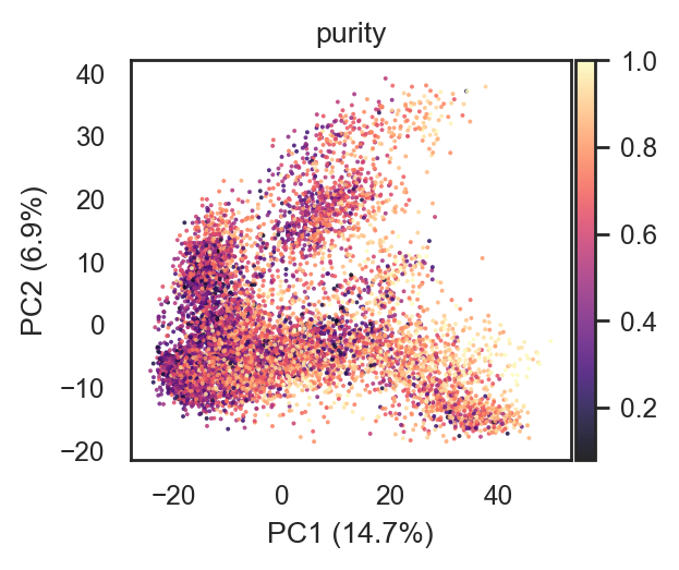
(<Figure size 600x500 with 2 Axes>,
 [<Axes: title={'center': 'purity'}, xlabel='PC1 (14.7%)', ylabel='PC2 (6.9%)'>])
bk.pl.pca_scatter(adata, color=["DLL3","SOX2","CDC20"], layer="log1p_cpm", point_size=8)
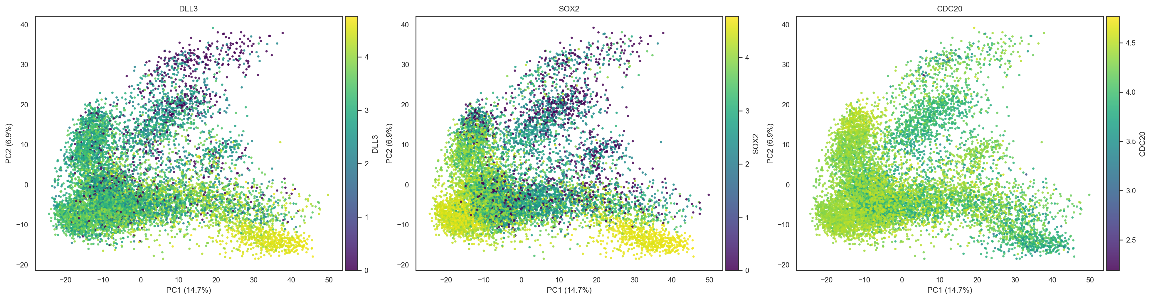
(<Figure size 3900x1000 with 6 Axes>,
 array([<Axes: title={'center': 'DLL3'}, xlabel='PC1 (14.7%)', ylabel='PC2 (6.9%)'>,
        <Axes: title={'center': 'SOX2'}, xlabel='PC1 (14.7%)', ylabel='PC2 (6.9%)'>,
        <Axes: title={'center': 'CDC20'}, xlabel='PC1 (14.7%)', ylabel='PC2 (6.9%)'>],
       dtype=object))
PCA Variance#
# 4) scree
bk.pl.pca_variance_ratio(adata,  figsize=(3, 2.5),
                         save= DESKTOP + "pca_variance_ratio_example.png")
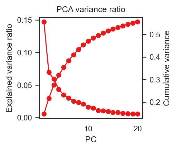
(<Figure size 600x500 with 2 Axes>,
 <Axes: title={'center': 'PCA variance ratio'}, xlabel='PC', ylabel='Explained variance ratio'>)
#If you ever call PCA with key_added=”pca_hvg”, then: bk.pl.pca_variance_ratio(adata, key=”pca_hvg”)
4.2. PCA loadings#
bk.tl.pca_loadings(adata, pcs=[1,2], n_top=5)
{'PC1_pos':         pc sign  rank        gene   loading
 15429  PC1  pos     1      PANTR1  0.050513
 10009  PC1  pos     2      ETNPPL  0.038816
 11731  PC1  pos     3      ARPP21  0.038311
 14450  PC1  pos     4      POU3F3  0.038200
 15903  PC1  pos     5  MIR124-1HG  0.035688,
 'PC1_neg':         pc sign  rank       gene   loading
 2889   PC1  neg     1    CEACAM5 -0.085973
 6766   PC1  neg     2     FGFBP1 -0.080500
 16022  PC1  neg     3  MIR200CHG -0.080387
 16265  PC1  neg     4    SLC6A14 -0.078849
 14780  PC1  neg     5   SERPINB5 -0.078713,
 'PC2_pos':         pc sign  rank     gene   loading
 6377   PC2  pos     1   UGT2A3  0.131476
 7949   PC2  pos     2  SLC17A4  0.125180
 5082   PC2  pos     3  SLC17A1  0.103836
 16413  PC2  pos     4    CCL15  0.101314
 9853   PC2  pos     5   SLC2A2  0.101277,
 'PC2_neg':         pc sign  rank      gene   loading
 10795  PC2  neg     1      KLK5 -0.075238
 15354  PC2  neg     2  MIR205HG -0.074715
 2303   PC2  neg     3     RIMS4 -0.070970
 9756   PC2  neg     4       IVL -0.062053
 6870   PC2  neg     5     CLCA2 -0.060242}
#Export
bk.tl.pca_loadings(
    adata,
    pcs=[1,2,3,4,5],
    n_top=100,
    export=DESKTOP + "TCGA_pca_loadings.tsv",
    export_gmt=DESKTOP + "TCGA_pca_loadings.gmt",
)
{'PC1_pos':         pc sign  rank        gene   loading
 15429  PC1  pos     1      PANTR1  0.050513
 10009  PC1  pos     2      ETNPPL  0.038816
 11731  PC1  pos     3      ARPP21  0.038311
 14450  PC1  pos     4      POU3F3  0.038200
 15903  PC1  pos     5  MIR124-1HG  0.035688
 ...    ...  ...   ...         ...       ...
 12621  PC1  pos    96      SERTM1  0.010446
 11326  PC1  pos    97        CDH2  0.010390
 13042  PC1  pos    98         UTY  0.010318
 5792   PC1  pos    99      TXLNGY  0.010153
 11315  PC1  pos   100      LONRF2  0.010115

 [100 rows x 5 columns],
 'PC1_neg':         pc sign  rank       gene   loading
 2889   PC1  neg     1    CEACAM5 -0.085973
 6766   PC1  neg     2     FGFBP1 -0.080500
 16022  PC1  neg     3  MIR200CHG -0.080387
 16265  PC1  neg     4    SLC6A14 -0.078849
 14780  PC1  neg     5   SERPINB5 -0.078713
 ...    ...  ...   ...        ...       ...
 14821  PC1  neg    96   IGLV4-69 -0.053010
 15631  PC1  neg    97   IGKV2-24 -0.052611
 2068   PC1  neg    98     PLA2G3 -0.052481
 15062  PC1  neg    99     MUC5AC -0.052362
 15643  PC1  neg   100    IGKV1-9 -0.052201

 [100 rows x 5 columns],
 'PC2_pos':         pc sign  rank     gene   loading
 6377   PC2  pos     1   UGT2A3  0.131476
 7949   PC2  pos     2  SLC17A4  0.125180
 5082   PC2  pos     3  SLC17A1  0.103836
 16413  PC2  pos     4    CCL15  0.101314
 9853   PC2  pos     5   SLC2A2  0.101277
 ...    ...  ...   ...      ...       ...
 5619   PC2  pos    96   RPS4Y1  0.039264
 6206   PC2  pos    97     REG4  0.038864
 15313  PC2  pos    98     ORM1  0.038812
 6252   PC2  pos    99    CFHR5  0.038626
 4510   PC2  pos   100      GDA  0.038363

 [100 rows x 5 columns],
 'PC2_neg':         pc sign  rank       gene   loading
 10795  PC2  neg     1       KLK5 -0.075238
 15354  PC2  neg     2   MIR205HG -0.074715
 2303   PC2  neg     3      RIMS4 -0.070970
 9756   PC2  neg     4        IVL -0.062053
 6870   PC2  neg     5      CLCA2 -0.060242
 ...    ...  ...   ...        ...       ...
 3474   PC2  neg    96      CCKBR -0.036507
 15171  PC2  neg    97  LINC01527 -0.036460
 1252   PC2  neg    98     CACNG4 -0.036313
 16203  PC2  neg    99    ANXA8L1 -0.036256
 2668   PC2  neg   100      AP3B2 -0.036214

 [100 rows x 5 columns],
 'PC3_pos':         pc sign  rank       gene   loading
 14510  PC3  pos     1     SPRR2E  0.048274
 16059  PC3  pos     2  LINC00520  0.044933
 15118  PC3  pos     3     MAGEA3  0.044752
 9755   PC3  pos     4      LCE3D  0.043588
 13967  PC3  pos     5     SPRR2B  0.042600
 ...    ...  ...   ...        ...       ...
 15586  PC3  pos    96   IGKV3-20  0.023137
 14841  PC3  pos    97   IGLV2-14  0.023044
 14830  PC3  pos    98   IGLV1-44  0.022944
 14847  PC3  pos    99      IGLC3  0.022920
 13213  PC3  pos   100      KRT76  0.022868

 [100 rows x 5 columns],
 'PC3_neg':         pc sign  rank         gene   loading
 15992  PC3  neg     1         RMST -0.101496
 11651  PC3  neg     2         FUT9 -0.085066
 1407   PC3  neg     3         SCGN -0.084644
 123    PC3  neg     4         TAC1 -0.082746
 15817  PC3  neg     5  C8orf34-AS1 -0.081935
 ...    ...  ...   ...          ...       ...
 8403   PC3  neg    96        FREM2 -0.050257
 5384   PC3  neg    97       TSPAN8 -0.050060
 8226   PC3  neg    98        HABP2 -0.050041
 2539   PC3  neg    99        OLFM4 -0.049925
 2333   PC3  neg   100       CHRNA4 -0.049919

 [100 rows x 5 columns],
 'PC4_pos':         pc sign  rank       gene   loading
 14346  PC4  pos     1     EIF1AY  0.115028
 5619   PC4  pos     2     RPS4Y1  0.113017
 13042  PC4  pos     3        UTY  0.111371
 972    PC4  pos     4        ZFY  0.110368
 5792   PC4  pos     5     TXLNGY  0.110098
 ...    ...  ...   ...        ...       ...
 15744  PC4  pos    96     UGT1A4  0.046672
 15188  PC4  pos    97  LINC00320  0.046622
 13520  PC4  pos    98     VSTM2B  0.046521
 9231   PC4  pos    99     HOXB13  0.046506
 13960  PC4  pos   100     POU3F4  0.046201

 [100 rows x 5 columns],
 'PC4_neg':         pc sign  rank       gene   loading
 15488  PC4  neg     1   nan-4509 -0.091501
 5129   PC4  neg     2    SCGB1D2 -0.081187
 16268  PC4  neg     3  nan-12819 -0.079381
 3507   PC4  neg     4    SCGB2A2 -0.076360
 5130   PC4  neg     5    SCGB2A1 -0.074540
 ...    ...  ...   ...        ...       ...
 10672  PC4  neg    96     PRR15L -0.030262
 14877  PC4  neg    97   IGHV3-23 -0.030059
 14841  PC4  neg    98   IGLV2-14 -0.029936
 16081  PC4  neg    99   ARNT2-DT -0.029799
 14832  PC4  neg   100   IGLV1-40 -0.029742

 [100 rows x 5 columns],
 'PC5_pos':         pc sign  rank         gene   loading
 14870  PC5  pos     1      IGHV3-7  0.110194
 16438  PC5  pos     2      IGHV4-4  0.109261
 15696  PC5  pos     3     IGKV1-12  0.097538
 14866  PC5  pos     4      IGHV6-1  0.097397
 16072  PC5  pos     5  IGHV1OR15-2  0.094806
 ...    ...  ...   ...          ...       ...
 10083  PC5  pos    96      TMEM174  0.050428
 949    PC5  pos    97        DDX3Y  0.050412
 4945   PC5  pos    98       HOXC13  0.050084
 3049   PC5  pos    99       PTPRZ1  0.049867
 16017  PC5  pos   100       SLC5A8  0.049222

 [100 rows x 5 columns],
 'PC5_neg':         pc sign  rank       gene   loading
 5737   PC5  neg     1    RBBP8NL -0.067558
 9336   PC5  neg     2       TFF1 -0.066807
 16022  PC5  neg     3  MIR200CHG -0.066354
 14384  PC5  neg     4       MUC2 -0.060665
 13155  PC5  neg     5     LRRC26 -0.059625
 ...    ...  ...   ...        ...       ...
 1588   PC5  neg    96      IGSF9 -0.024556
 5580   PC5  neg    97      AP1M2 -0.024544
 3382   PC5  neg    98      CWH43 -0.024517
 11940  PC5  neg    99     GOLT1A -0.024057
 2654   PC5  neg   100       TMC5 -0.023699

 [100 rows x 5 columns]}
#Absolute loadings only (single list per PC)
bk.tl.pca_loadings(adata, pcs=[1,2,3], n_top=100, use_abs=True)
{'PC1_abs':         pc sign  rank      gene   loading
 50438  PC1  abs     1   CEACAM6 -0.086779
 8052   PC1  abs     2     KRT6A -0.084907
 50435  PC1  abs     3   CEACAM5 -0.083953
 16858  PC1  abs     4      AGR2 -0.081556
 2256   PC1  abs     5  SERPINB5 -0.080948
 ...    ...  ...   ...       ...       ...
 46401  PC1  abs    96     ESRP2 -0.050246
 50860  PC1  abs    97      BCAN  0.050191
 28140  PC1  abs    98    S100A2 -0.049962
 18737  PC1  abs    99   ANXA8L1 -0.049845
 24337  PC1  abs   100     IGHA2 -0.049593

 [100 rows x 5 columns],
 'PC2_abs':         pc sign  rank     gene   loading
 40168  PC2  abs     1    HNF4A -0.099591
 11245  PC2  abs     2    CDHR5 -0.089164
 52362  PC2  abs     3    ALDOB -0.088794
 20467  PC2  abs     4     A1CF -0.087727
 6005   PC2  abs     5      FGA -0.085978
 ...    ...  ...   ...      ...       ...
 5772   PC2  abs    96   CYP3A5 -0.055155
 10653  PC2  abs    97  UGT2B15 -0.055070
 15896  PC2  abs    98   UGT3A1 -0.055053
 32526  PC2  abs    99    ADH1B -0.055015
 11040  PC2  abs   100      F11 -0.054943

 [100 rows x 5 columns],
 'PC3_abs':         pc sign  rank     gene   loading
 34663  PC3  abs     1  PPP1R1B -0.097308
 23941  PC3  abs     2    SPDEF -0.089340
 16859  PC3  abs     3     AGR3 -0.083124
 16858  PC3  abs     4     AGR2 -0.079345
 8050   PC3  abs     5    KRT6C  0.076780
 ...    ...  ...   ...      ...       ...
 33474  PC3  abs    96     DSG3  0.048774
 19029  PC3  abs    97    CLCA2  0.048597
 15785  PC3  abs    98    KCNC2 -0.048482
 7840   PC3  abs    99   PCDH10 -0.048453
 51691  PC3  abs   100    LCE3D  0.048305

 [100 rows x 5 columns]}
# Barplot for PC1 (top pos/neg)
bk.pl.pca_loadings_bar(adata, pc=1, n_top=10, figsize=(2.5,3),
                      save=DESKTOP + "pc1_loadings_bar.png")
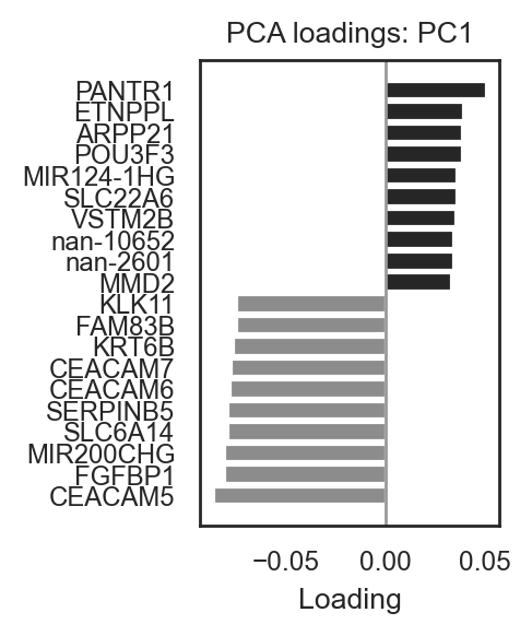
(<Figure size 500x600 with 1 Axes>,
 <Axes: title={'center': 'PCA loadings: PC1'}, xlabel='Loading'>)
# Barplot for PC2 (top pos/neg)
bk.pl.pca_loadings_bar(adata, pc=2, n_top=10, figsize=(2.5,3),
                      save=DESKTOP + "pc2_loadings_bar.png")
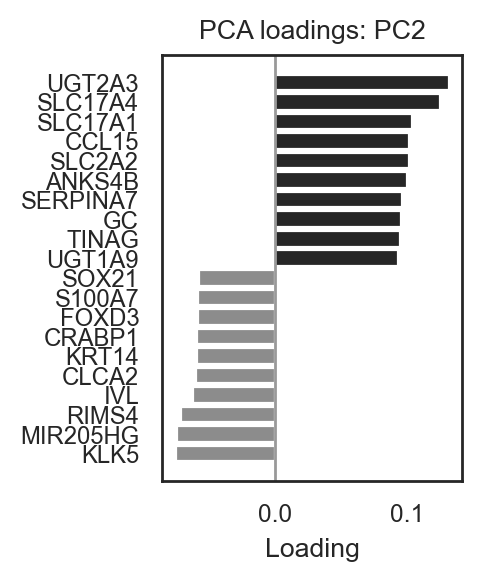
(<Figure size 500x600 with 1 Axes>,
 <Axes: title={'center': 'PCA loadings: PC2'}, xlabel='Loading'>)
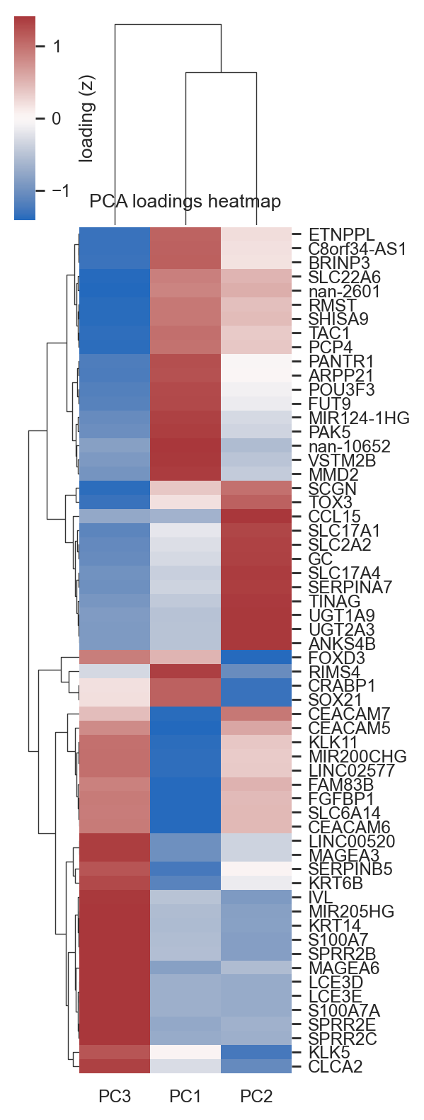
# Heatmap for PC1–PC5 (union of top genes)
bk.pl.pca_loadings_heatmap(
    adata,
    pcs=[1,2,3],
    n_top=10,
    cluster_genes=True,
    cluster_pcs=True,
    z_score=True,
    figsize=(3,8),
    save=DESKTOP + "pca_loadings_heatmap_TCGAall.png",
);
4.3. Neighbors & UMAP#
Common bulk-friendly parameter ranges • n_neighbors: 10–30 (for ~100 samples, 15 is a good start) • resolution: • 0.3–0.8 for broader groups • 1.0–2.0 for finer subclusters
# Calculate neighbors - PCA should be already computed
bk.tl.neighbors(adata, n_neighbors=15, n_pcs=20, metric="euclidean")
bk.tl.umap(adata, n_neighbors=8, n_pcs=30, min_dist=0.3, random_state=0) #0.3
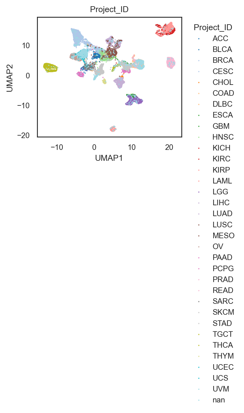
bk.pl.umap(adata, color="Project_ID",
           figsize=(3,3),
           point_size=2, palette="tab20",               # palette "husl".. others
           save=DESKTOP + "UMAP_ProjectID.png")
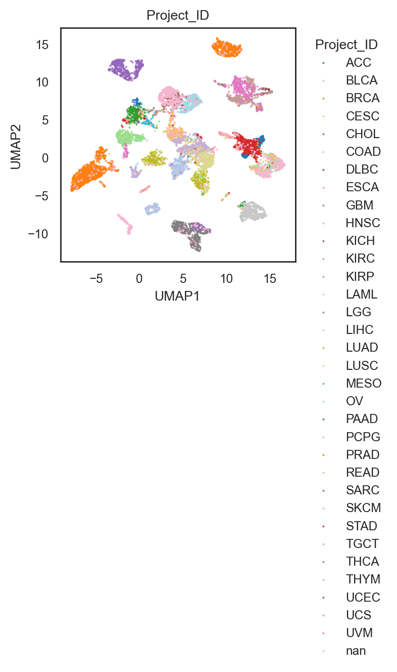
(<Figure size 600x600 with 1 Axes>,
 [<Axes: title={'center': 'Project_ID'}, xlabel='UMAP1', ylabel='UMAP2'>])
# gene expression (continuous, from a layer)
bk.pl.umap(adata, color="DLL3", layer="log1p_cpm", figsize=(3,2.5), point_size=5,
          save=DESKTOP + "UMAP_DLL3.png")   #cmap="magma"
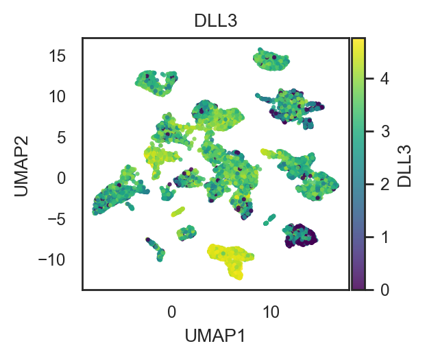
(<Figure size 600x500 with 2 Axes>,
 [<Axes: title={'center': 'DLL3'}, xlabel='UMAP1', ylabel='UMAP2'>])
# continuous metadata
bk.pl.umap(adata, color="Age at Diagnosis in Years",
           figsize=(3,2.5), point_size=2,
           cmap="viridis")
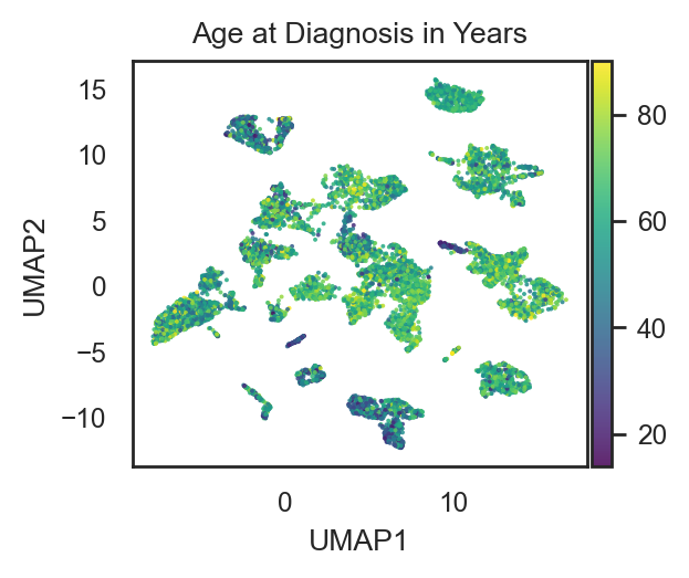
(<Figure size 600x500 with 2 Axes>,
 [<Axes: title={'center': 'Age at Diagnosis in Years'}, xlabel='UMAP1', ylabel='UMAP2'>])
# continuous metadata
bk.pl.umap(adata, color="purity",
           figsize=(3,2.5), point_size=2,
           cmap="magma",
          save=DESKTOP + "UMAP_purity_magma.png")
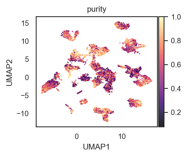
(<Figure size 600x500 with 2 Axes>,
 [<Axes: title={'center': 'purity'}, xlabel='UMAP1', ylabel='UMAP2'>])
# multiple genes → 1 row of panels
bk.pl.umap(adata, color=["GFAP", "OLIG1", "DLL3"], layer="log1p_cpm",
           figsize=(3,2.5),
           point_size=8, cmap="viridis",
          save=DESKTOP + "umap_genes_example.png")
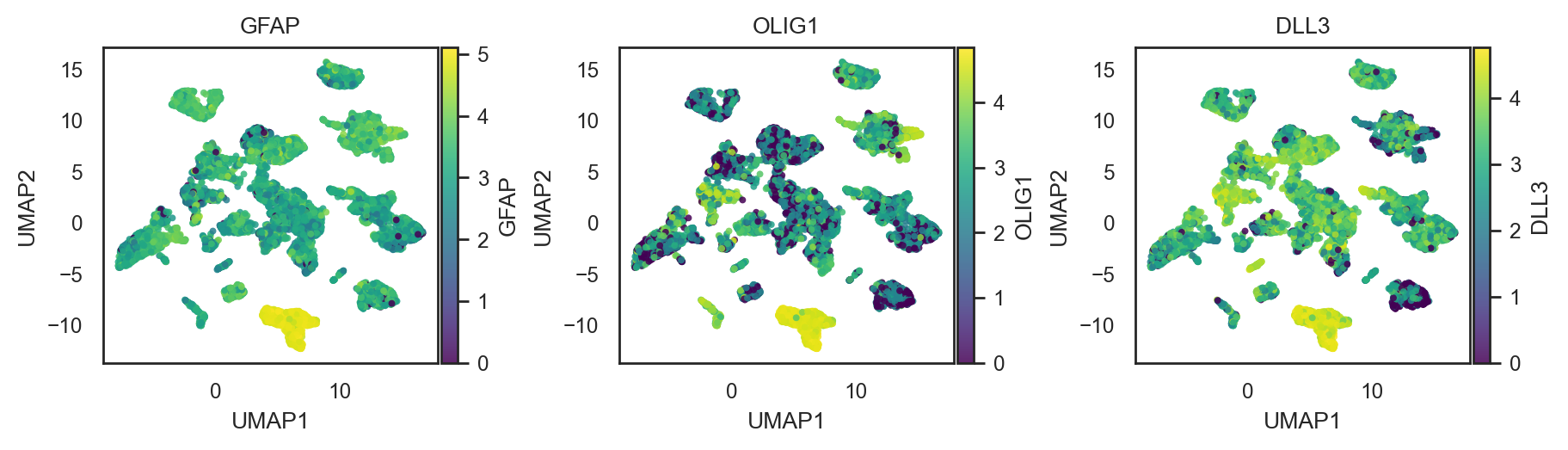
(<Figure size 1800x500 with 6 Axes>,
 array([<Axes: title={'center': 'GFAP'}, xlabel='UMAP1', ylabel='UMAP2'>,
        <Axes: title={'center': 'OLIG1'}, xlabel='UMAP1', ylabel='UMAP2'>,
        <Axes: title={'center': 'DLL3'}, xlabel='UMAP1', ylabel='UMAP2'>],
       dtype=object))
Compare umap & umap_graph:#
umap: regular, representation-driven, standard
umap_graph: “Graph-enforced UMAP reveals subtype separation”, topology-preserving, exploratory
Original:
min_dist=0.3,
random_state=0,
bk.tl.umap_graph(
    adata,
    graph_key="connectivities",
    min_dist=0.5,
    random_state=0,
)
bk.pl.umap(adata, basis="X_umap_graph", color="Project_ID", figsize=(3,2.5), point_size=2, palette="Set20")
(<Figure size 600x500 with 1 Axes>,
 [<Axes: title={'center': 'Project_ID'}, xlabel='UMAP1', ylabel='UMAP2'>])
Save bidimensional representation X,Y values#
adata.write("../data/h5ad/260127_TCGA_example_in_BULLKpy.h5ad", compression="gzip")
5. Clustering and define groups #
Basic procedure: PCA → 2) neighbors graph on PCs → 3) Leiden (scan resolution)
Use
method=leidenfor computational of clusters.resolution: Higher resolution → more clusters // Lower resolution → fewer clusters. Leiden requires a graph, so run afterbk.tl.neighbors(already computed for UMAP)Use K-means when you want direct control over the number of clusters or a quick baseline.
Try Leiden; if not installed it will fallback to kmeans automatically
5.1. Leiden#
For complex structure and unknown number of clusters
# Initial test if true groups already known. Scan many Leiden resolutions
df = bk.tl.leiden_resolution_scan(
    adata,
    true_key="Project_ID",                                          # Biological true groups
    resolutions=[0.4, 0.6, 0.8, 1.0, 1.5],
    base_key="leiden",
    use_rep="X_pca",
    n_pcs=20,
    n_neighbors=15,
)
df
| resolution | key | n_clusters | ARI | NMI | cramers_v | n_used | n_missing | |
|---|---|---|---|---|---|---|---|---|
| 0 | 0.4 | leiden_0.4 | 16 | 0.647859 | 0.832598 | 0.967372 | 10120 | 937 |
| 1 | 0.6 | leiden_0.6 | 20 | 0.660811 | 0.835409 | 0.906566 | 10120 | 937 |
| 2 | 0.8 | leiden_0.8 | 24 | 0.698434 | 0.841443 | 0.870219 | 10120 | 937 |
| 3 | 1.0 | leiden_1 | 26 | 0.671333 | 0.831292 | 0.831609 | 10120 | 937 |
| 4 | 1.5 | leiden_1.5 | 33 | 0.659986 | 0.825683 | 0.774511 | 10120 | 937 |
# Heatmap of ARI vs resolution in the previous calculations
bk.pl.ari_resolution_heatmap(
    adata,
    df=df,
    metric="ARI",
    show_n_clusters=True,
    figsize=(4,2)
    #save="figs/ari_vs_resolution.png",
)
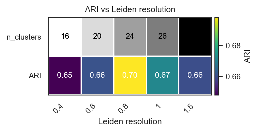
(<Figure size 800x400 with 2 Axes>,
 <Axes: title={'center': 'ARI vs Leiden resolution'}, xlabel='Leiden resolution'>)
# A single calculation with a specific resolution
bk.tl.cluster(adata, method="leiden", key_added="leiden_0.8", resolution=0.8)
# Ensure data are taken as categorical, not numeric
adata.obs["leiden_2.2"] = adata.obs["leiden_2.2"].astype("category")
bk.pl.pca_scatter(adata, color="leiden_0.8",
                  figsize=(2.8,2.5),                           # figsize=(3.5,3.5)
                  point_size=5)    #save="pca_clusters.png"
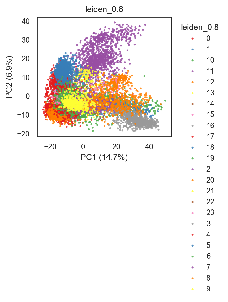
(<Figure size 560x500 with 1 Axes>,
 [<Axes: title={'center': 'leiden_0.8'}, xlabel='PC1 (14.7%)', ylabel='PC2 (6.9%)'>])
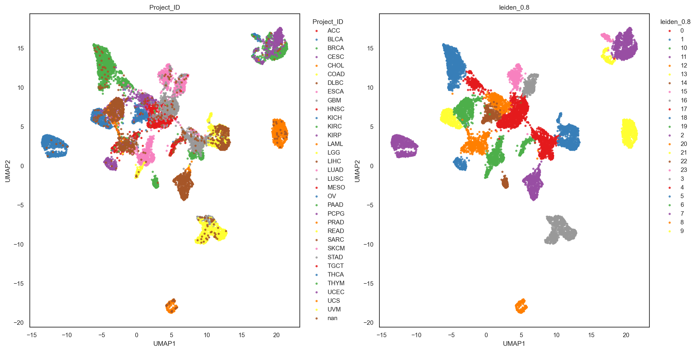
bk.pl.umap(adata, color=["Project_ID", "leiden_0.8"],
           figsize=(3,2.5),
           point_size=2,
           save=DESKTOP + "UMAP_lein0.8_example.png")
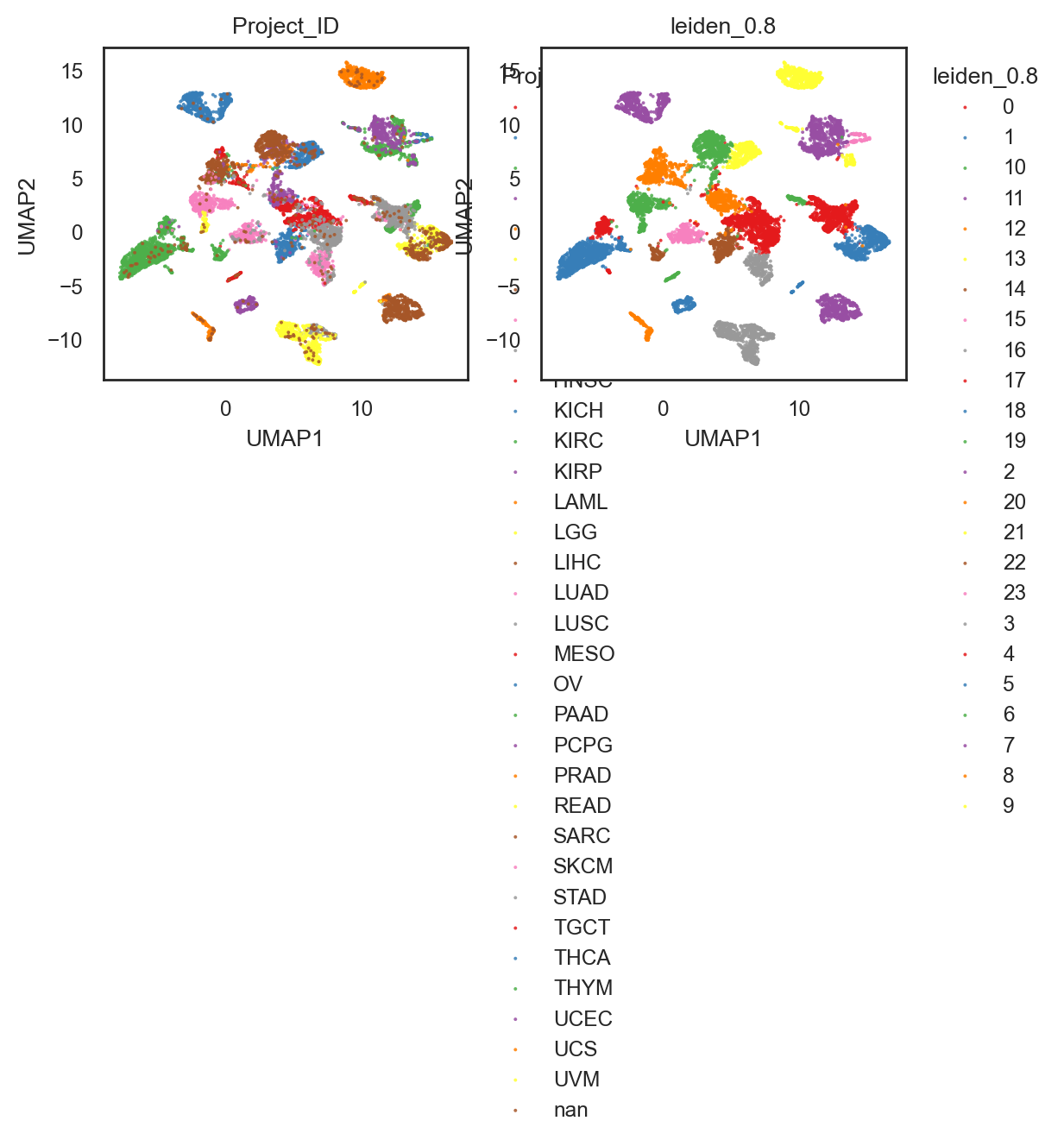
(<Figure size 1200x500 with 2 Axes>,
 array([<Axes: title={'center': 'Project_ID'}, xlabel='UMAP1', ylabel='UMAP2'>,
        <Axes: title={'center': 'leiden_0.8'}, xlabel='UMAP1', ylabel='UMAP2'>],
       dtype=object))
bk.pl.pca_scatter(adata, color=["Project_ID", "leiden_0.8"],
                  figsize=(3,2.5),
                  point_size=2,
                  save=DESKTOP + "UMAP_lein0.8_example.png")
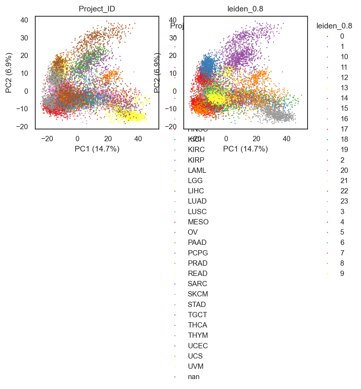
(<Figure size 1200x500 with 2 Axes>,
 array([<Axes: title={'center': 'Project_ID'}, xlabel='PC1 (14.7%)', ylabel='PC2 (6.9%)'>,
        <Axes: title={'center': 'leiden_0.8'}, xlabel='PC1 (14.7%)', ylabel='PC2 (6.9%)'>],
       dtype=object))
bk.pl.umap(adata, basis="X_umap", color=["Project_ID", "leiden_0.8"], figsize=(7,7), point_size=10)             #save="umap_leiden_standard.png"
bk.pl.umap(adata, basis="X_umap_graph", color=["Project_ID", "leiden_0.8"], figsize=(7,7), point_size=10)      #save="umap_leiden_standard.png"
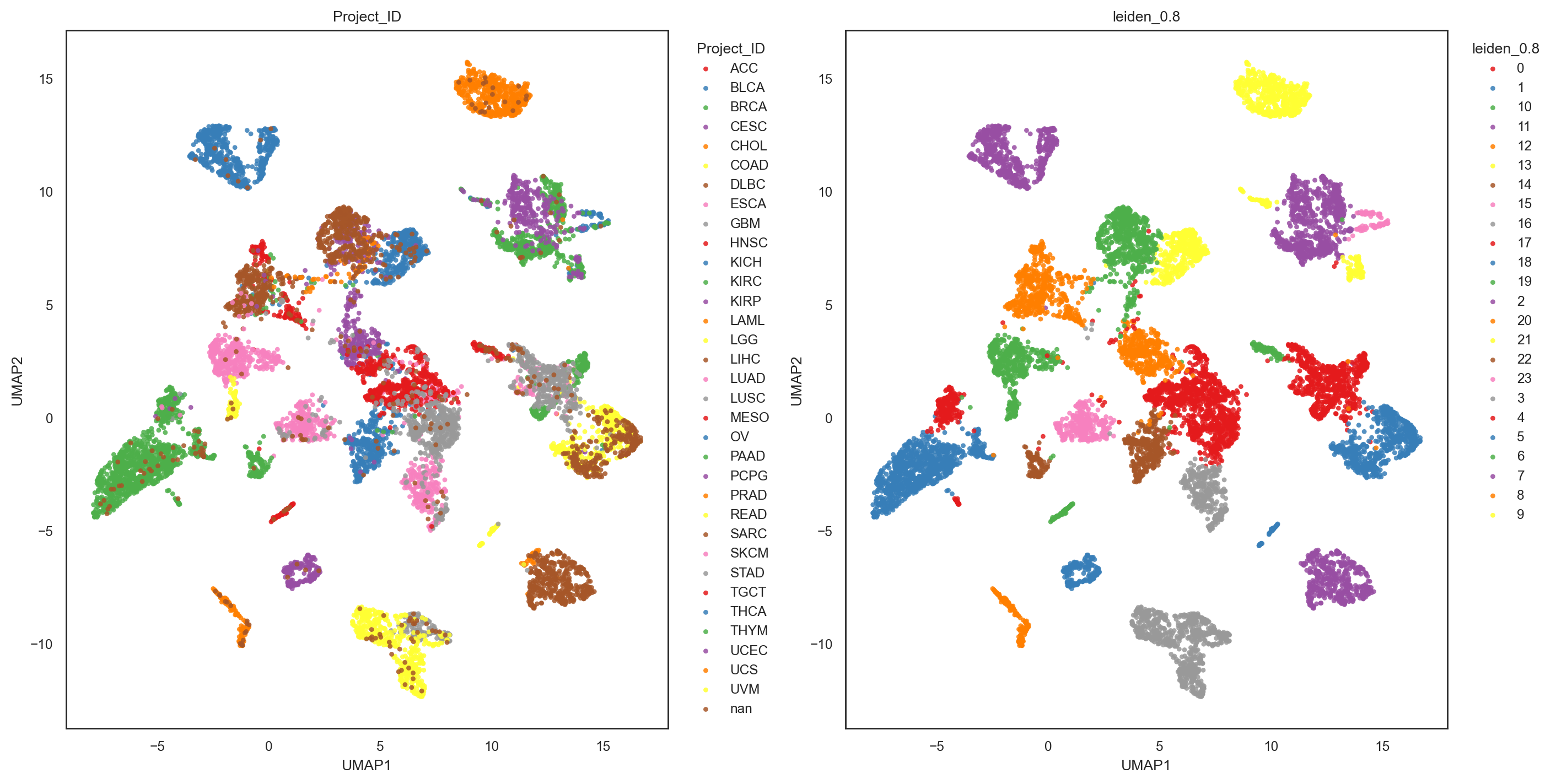
(<Figure size 2800x1400 with 2 Axes>,
 array([<Axes: title={'center': 'Project_ID'}, xlabel='UMAP1', ylabel='UMAP2'>,
        <Axes: title={'center': 'leiden_0.8'}, xlabel='UMAP1', ylabel='UMAP2'>],
       dtype=object))
# Compare results leiden vs. True biological
pd.crosstab(adata.obs["Project_ID"], adata.obs["leiden_2"])
| leiden_2 | 0 | 1 | 10 | 11 | 12 | 13 | 14 | 15 | 16 | 17 | ... | 33 | 34 | 35 | 36 | 4 | 5 | 6 | 7 | 8 | 9 |
|---|---|---|---|---|---|---|---|---|---|---|---|---|---|---|---|---|---|---|---|---|---|
| Project_ID | |||||||||||||||||||||
| ACC | 0 | 0 | 0 | 0 | 0 | 0 | 0 | 0 | 0 | 0 | ... | 0 | 0 | 0 | 0 | 0 | 0 | 75 | 0 | 0 | 0 |
| BLCA | 3 | 3 | 0 | 0 | 0 | 0 | 336 | 0 | 0 | 0 | ... | 0 | 0 | 0 | 0 | 0 | 0 | 11 | 32 | 0 | 6 |
| BRCA | 1 | 1 | 0 | 0 | 0 | 354 | 0 | 0 | 0 | 0 | ... | 0 | 0 | 0 | 21 | 498 | 1 | 15 | 7 | 0 | 0 |
| CESC | 4 | 15 | 0 | 1 | 0 | 0 | 1 | 0 | 0 | 0 | ... | 0 | 0 | 0 | 0 | 1 | 0 | 1 | 265 | 0 | 1 |
| CHOL | 3 | 0 | 0 | 0 | 0 | 0 | 0 | 0 | 0 | 0 | ... | 0 | 0 | 0 | 0 | 0 | 41 | 1 | 0 | 0 | 0 |
| COAD | 5 | 0 | 0 | 0 | 0 | 0 | 0 | 154 | 0 | 0 | ... | 0 | 0 | 41 | 0 | 0 | 0 | 0 | 0 | 0 | 0 |
| DLBC | 2 | 0 | 1 | 0 | 0 | 0 | 0 | 0 | 0 | 0 | ... | 0 | 0 | 0 | 0 | 0 | 0 | 41 | 0 | 0 | 0 |
| ESCA | 81 | 0 | 0 | 0 | 0 | 0 | 0 | 0 | 0 | 0 | ... | 0 | 0 | 0 | 0 | 0 | 0 | 0 | 1 | 0 | 3 |
| GBM | 0 | 0 | 0 | 0 | 0 | 0 | 0 | 0 | 0 | 0 | ... | 0 | 0 | 0 | 0 | 0 | 0 | 0 | 0 | 0 | 0 |
| HNSC | 0 | 0 | 0 | 0 | 0 | 0 | 0 | 0 | 0 | 0 | ... | 0 | 0 | 0 | 0 | 0 | 0 | 1 | 117 | 1 | 7 |
| KICH | 0 | 0 | 0 | 0 | 0 | 0 | 0 | 0 | 0 | 0 | ... | 63 | 0 | 0 | 0 | 0 | 0 | 2 | 0 | 0 | 0 |
| KIRC | 2 | 0 | 0 | 0 | 331 | 0 | 0 | 0 | 0 | 0 | ... | 12 | 0 | 0 | 0 | 0 | 0 | 4 | 0 | 0 | 0 |
| KIRP | 0 | 0 | 0 | 0 | 40 | 0 | 4 | 0 | 0 | 0 | ... | 6 | 0 | 0 | 0 | 0 | 0 | 0 | 0 | 0 | 0 |
| LAML | 0 | 0 | 0 | 0 | 0 | 0 | 0 | 0 | 0 | 0 | ... | 0 | 0 | 0 | 0 | 0 | 0 | 0 | 0 | 0 | 0 |
| LGG | 0 | 0 | 0 | 0 | 0 | 0 | 0 | 0 | 0 | 0 | ... | 0 | 0 | 0 | 0 | 0 | 0 | 1 | 0 | 0 | 0 |
| LIHC | 1 | 0 | 0 | 0 | 0 | 0 | 0 | 0 | 0 | 0 | ... | 0 | 0 | 0 | 0 | 0 | 413 | 4 | 0 | 0 | 0 |
| LUAD | 1 | 2 | 0 | 0 | 0 | 0 | 1 | 0 | 259 | 286 | ... | 0 | 0 | 0 | 0 | 0 | 0 | 1 | 1 | 0 | 9 |
| LUSC | 1 | 1 | 0 | 0 | 0 | 0 | 1 | 0 | 56 | 29 | ... | 0 | 0 | 0 | 0 | 0 | 1 | 1 | 14 | 0 | 388 |
| MESO | 0 | 0 | 0 | 0 | 0 | 0 | 0 | 0 | 2 | 0 | ... | 0 | 0 | 0 | 0 | 0 | 0 | 3 | 0 | 0 | 1 |
| OV | 0 | 5 | 0 | 351 | 0 | 0 | 0 | 0 | 0 | 0 | ... | 0 | 0 | 0 | 0 | 0 | 0 | 1 | 0 | 0 | 0 |
| PAAD | 173 | 0 | 0 | 0 | 0 | 0 | 0 | 2 | 0 | 0 | ... | 0 | 0 | 0 | 0 | 0 | 0 | 5 | 1 | 0 | 0 |
| PCPG | 0 | 0 | 0 | 0 | 0 | 0 | 0 | 0 | 0 | 0 | ... | 0 | 0 | 0 | 0 | 0 | 0 | 2 | 0 | 0 | 0 |
| PRAD | 0 | 0 | 0 | 0 | 0 | 0 | 0 | 0 | 0 | 0 | ... | 0 | 0 | 0 | 0 | 0 | 0 | 0 | 0 | 0 | 0 |
| READ | 2 | 0 | 0 | 0 | 0 | 0 | 0 | 46 | 0 | 0 | ... | 0 | 0 | 10 | 0 | 0 | 1 | 0 | 0 | 0 | 0 |
| SARC | 2 | 1 | 0 | 0 | 0 | 0 | 0 | 0 | 1 | 0 | ... | 0 | 0 | 0 | 0 | 0 | 0 | 253 | 0 | 3 | 0 |
| SKCM | 0 | 2 | 0 | 0 | 0 | 0 | 0 | 0 | 3 | 0 | ... | 0 | 2 | 0 | 0 | 0 | 0 | 7 | 2 | 443 | 0 |
| STAD | 381 | 0 | 0 | 0 | 0 | 0 | 0 | 1 | 0 | 0 | ... | 0 | 0 | 1 | 0 | 0 | 1 | 3 | 0 | 0 | 1 |
| TGCT | 1 | 0 | 0 | 0 | 0 | 0 | 0 | 0 | 0 | 0 | ... | 0 | 0 | 0 | 0 | 0 | 0 | 0 | 0 | 0 | 0 |
| THCA | 0 | 0 | 407 | 0 | 0 | 0 | 0 | 0 | 0 | 0 | ... | 0 | 0 | 0 | 0 | 0 | 0 | 0 | 0 | 0 | 0 |
| THYM | 0 | 1 | 0 | 0 | 0 | 0 | 0 | 0 | 0 | 0 | ... | 0 | 0 | 0 | 0 | 0 | 0 | 0 | 0 | 0 | 4 |
| UCEC | 1 | 176 | 0 | 7 | 0 | 0 | 0 | 0 | 0 | 0 | ... | 0 | 0 | 0 | 0 | 0 | 0 | 4 | 2 | 0 | 0 |
| UCS | 0 | 43 | 0 | 1 | 0 | 0 | 0 | 0 | 0 | 0 | ... | 0 | 0 | 0 | 0 | 0 | 0 | 12 | 0 | 0 | 0 |
| UVM | 0 | 0 | 0 | 0 | 0 | 0 | 0 | 0 | 0 | 0 | ... | 0 | 70 | 0 | 0 | 0 | 0 | 0 | 0 | 5 | 0 |
33 rows × 37 columns
# estimate how good is the correlation - Compute ARI - NMI - cramers_v, silhouette
# ARI: from sklearn.metrics import adjusted_rand_score
# NMI: from sklearn.metrics import normalized_mutual_info_score

# Test1. One clustering vs ground truth (plus silhouette on PCA)
#bk.tl.neighbors(adata, n_neighbors=15, n_pcs=20)  # if not done
#bk.tl.leiden(adata, resolution=1.0)

m = bk.tl.cluster_metrics(
    adata,
    true_key="Project_ID",
    cluster_key="leiden_0.8",
    use_rep="X_pca",
    n_pcs=20,
)
m
{'n_used': 10120.0,
 'ari': 0.6984336007627627,
 'nmi': 0.8414429339645842,
 'cramers_v': 0.869389175552292,
 'silhouette': 0.2683062681973579}
# Plot results
bk.pl.ari_resolution_heatmap(adata, df=df, metric="NMI")
bk.pl.ari_resolution_heatmap(adata, df=df, metric="cramers_v")
#bk.pl.ari_resolution_heatmap(adata, df=df, metric="silhouette", vmin=None, vmax=None)
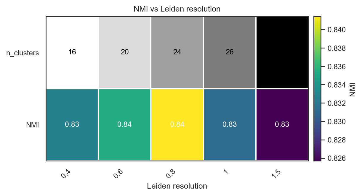
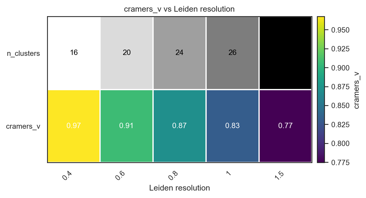
(<Figure size 1200x640 with 2 Axes>,
 <Axes: title={'center': 'cramers_v vs Leiden resolution'}, xlabel='Leiden resolution'>)
5.2. K-means#
Fixed number of clusters
# try several k values
for k in [10, 15, 20, 25, 30]:
    bk.tl.cluster(
        adata,
        method="kmeans",
        n_clusters=k,
        use_rep="X_pca",
        n_pcs=20,
        key_added=f"kmeans_{k}",
    )
# evaluate quantitively
bk.tl.cluster_metrics(
    adata,
    cluster_key="kmeans_25",
    true_key="Project_ID",
)
{'n_used': 10120.0,
 'ari': 0.6648309607082293,
 'nmi': 0.7929232959336532,
 'cramers_v': 0.7919848996323253,
 'silhouette': 0.2849268475400908}
# Calculate for a fixed number of clusters
bk.tl.cluster(
    adata,
    method="kmeans",
    n_clusters=25,
    use_rep="X_pca",
    n_pcs=20,
    key_added="kmeans_25",
    random_state=0,
)
bk.pl.pca_scatter(adata, color=["Project_ID", "kmeans_25"], figsize=(3,2.5), point_size=5,
                 save=DESKTOP + "PCA_kmeans_25.png")
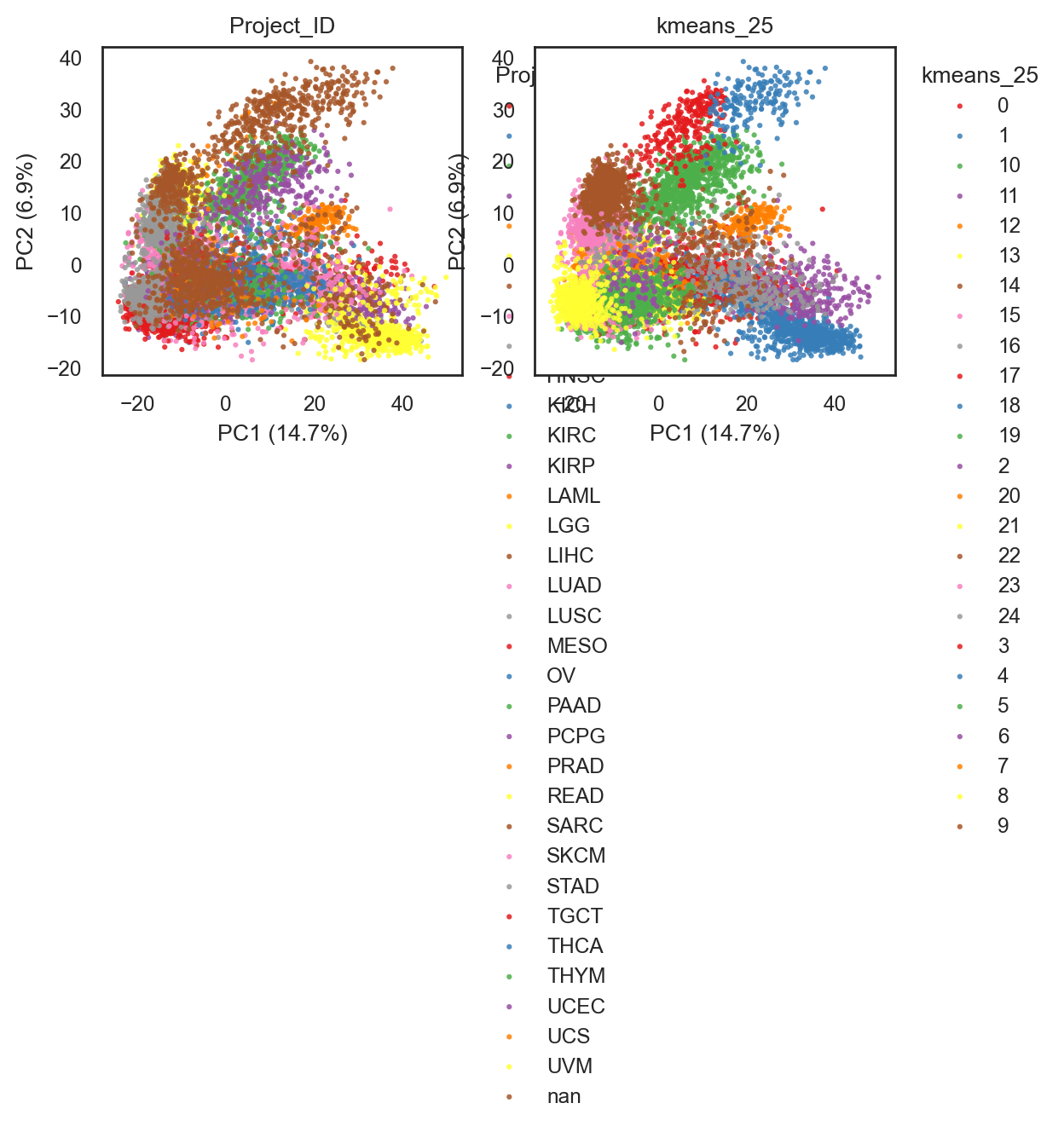
(<Figure size 1200x500 with 2 Axes>,
 array([<Axes: title={'center': 'Project_ID'}, xlabel='PC1 (14.7%)', ylabel='PC2 (6.9%)'>,
        <Axes: title={'center': 'kmeans_25'}, xlabel='PC1 (14.7%)', ylabel='PC2 (6.9%)'>],
       dtype=object))
bk.pl.umap(adata, color=["Project_ID", "kmeans_25"], figsize=(3.5,3), point_size=2,
          save=DESKTOP + "UMAP_kmeans_25.png")
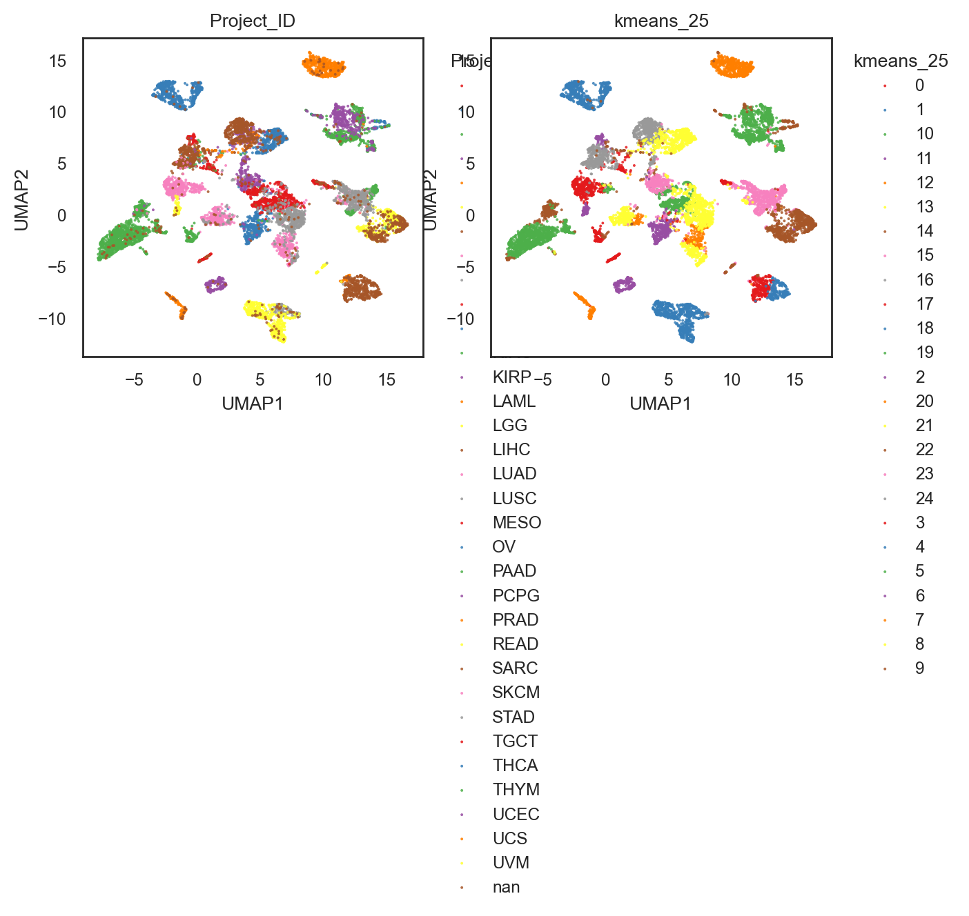
(<Figure size 1400x600 with 2 Axes>,
 array([<Axes: title={'center': 'Project_ID'}, xlabel='UMAP1', ylabel='UMAP2'>,
        <Axes: title={'center': 'kmeans_25'}, xlabel='UMAP1', ylabel='UMAP2'>],
       dtype=object))
# save .h5ad file
adata.write("../data/h5ad/260127_TCGA_example_in_BULLKpy.h5ad", compression="gzip")
6. Genes and Gene Signatures#
6.1. Gene plots#
bk.pl.pca_scatter(adata, color=["CDC20", "ASCL1","CD3D"],)
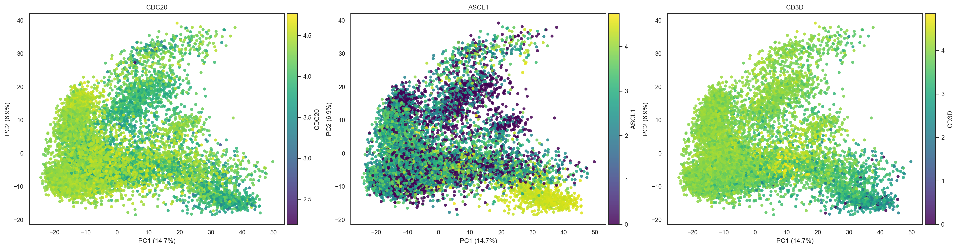
(<Figure size 3900x1000 with 6 Axes>,
 array([<Axes: title={'center': 'CDC20'}, xlabel='PC1 (14.7%)', ylabel='PC2 (6.9%)'>,
        <Axes: title={'center': 'ASCL1'}, xlabel='PC1 (14.7%)', ylabel='PC2 (6.9%)'>,
        <Axes: title={'center': 'CD3D'}, xlabel='PC1 (14.7%)', ylabel='PC2 (6.9%)'>],
       dtype=object))
bk.pl.violin(
    adata,
    keys=["MKI67", "DLL3"],
    groupby="Project_ID",
    #layer="log1p_cpm",      # or "counts" / None
    rotate_xticks=90,
    figsize=(8, 2.5),
    save=DESKTOP + "violin_Ki67_DLL3.png",
)
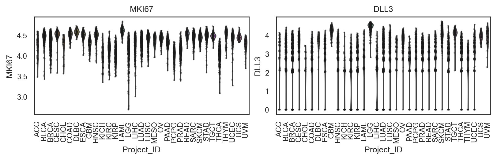
(<Figure size 1600x500 with 2 Axes>,
 array([<Axes: title={'center': 'MKI67'}, xlabel='Project_ID', ylabel='MKI67'>,
        <Axes: title={'center': 'DLL3'}, xlabel='Project_ID', ylabel='DLL3'>],
       dtype=object))
6.2. Score gene signatures#
6.2.1. A dictionary of signatures#
# Define signatures
signatures = {
    "Proliferation": ["MKI67", "TOP2A", "CDC20", "CCNB1", "CCNDA2"],
    "T_cell": ["CD3D", "CD3E", "TRBC1"],
    "Neuroendocrine": ["ASCL1", "NEUROD1", "DLL3", "CHGA"],
}
# Compute signature scores
bk.tl.score_genes_dict(
    adata,
    signatures,
    layer="log1p_cpm",
    scale=True,
)
bk.pl.pca_scatter(
    adata,
    color=["Proliferation_score", "Neuroendocrine_score"],
    cmap="viridis",
    figsize=(3.4,3),
    point_size=2,
    save=DESKTOP + "PCA_signatures_example.png",
)
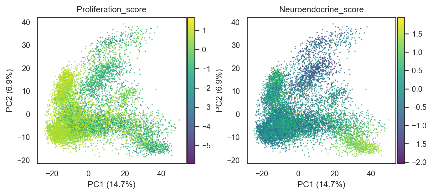
(<Figure size 1360x600 with 4 Axes>,
 array([<Axes: title={'center': 'Proliferation_score'}, xlabel='PC1 (14.7%)', ylabel='PC2 (6.9%)'>,
        <Axes: title={'center': 'Neuroendocrine_score'}, xlabel='PC1 (14.7%)', ylabel='PC2 (6.9%)'>],
       dtype=object))
adata.obs.head(3)
| Sample_ID | Patient_ID | Project_ID | gender | race | ajcc_pathologic_tumor_stage | clinical_stage | histological_type | histological_grade | initial_pathologic_dx_year | ... | SOX2_mut | ASCL1_mut | NEUROD1_mut | POU2F3_mut | YAP1_mut | NE25_score | total_counts | pct_counts_mt | libsize | leiden_2.5 | |
|---|---|---|---|---|---|---|---|---|---|---|---|---|---|---|---|---|---|---|---|---|---|
| TCGA-OR-A5JP-01A | TCGA-OR-A5JP-01 | TCGA-OR-A5JP | ACC | MALE | WHITE | Stage II | NaN | Adrenocortical carcinoma- Usual Type | NaN | 2012.0 | ... | 0.0 | 0.0 | 0.0 | 0.0 | 0.0 | NaN | 134123 | 0.196089 | 134123.0 | 5 |
| TCGA-OR-A5JG-01A | TCGA-OR-A5JG-01 | TCGA-OR-A5JG | ACC | MALE | WHITE | Stage IV | NaN | Adrenocortical carcinoma- Usual Type | NaN | 2008.0 | ... | 0.0 | 0.0 | 0.0 | 0.0 | 0.0 | NaN | 129774 | 0.209595 | 129774.0 | 5 |
| TCGA-OR-A5K1-01A | TCGA-OR-A5K1-01 | TCGA-OR-A5K1 | ACC | MALE | WHITE | Stage II | NaN | Adrenocortical carcinoma- Usual Type | NaN | 2006.0 | ... | 0.0 | 0.0 | 0.0 | 0.0 | 0.0 | NaN | 120282 | 0.229461 | 120282.0 | 5 |
3 rows × 1120 columns
bk.pl.pca_scatter(
    adata,
    color=["MKI67"],
    cmap="viridis",
    figsize=(3.4,3),
    point_size=2,
)
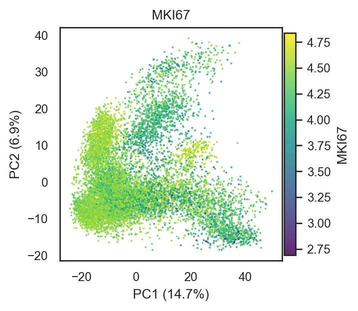
(<Figure size 680x600 with 2 Axes>,
 [<Axes: title={'center': 'MKI67'}, xlabel='PC1 (14.7%)', ylabel='PC2 (6.9%)'>])
bk.pl.violin(
    adata,
    keys=["Proliferation_score", "Neuroendocrine_score"],
    groupby="Project_ID",
    figsize=(8,2.5),
    rotate_xticks=90,
    save=DESKTOP + "violin_signatures_example.png",
)
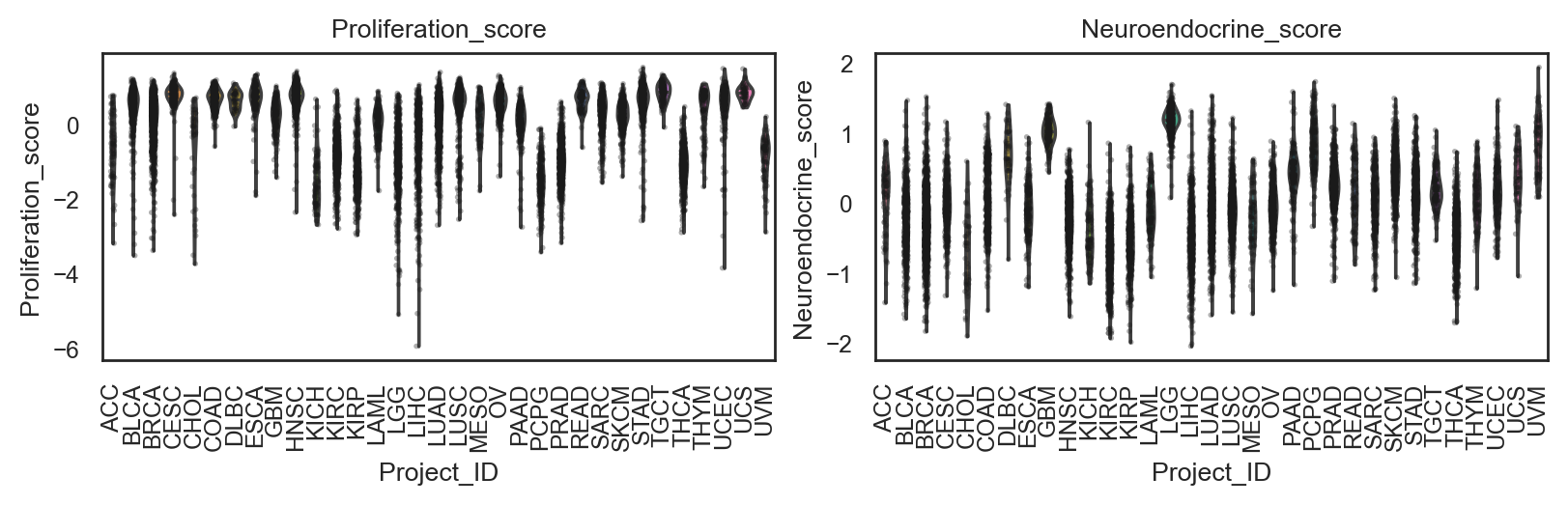
(<Figure size 1600x500 with 2 Axes>,
 array([<Axes: title={'center': 'Proliferation_score'}, xlabel='Project_ID', ylabel='Proliferation_score'>,
        <Axes: title={'center': 'Neuroendocrine_score'}, xlabel='Project_ID', ylabel='Neuroendocrine_score'>],
       dtype=object))
6.2.2. A single signature#
ne_score_25 = ['BEX1', 'ASCL1', 'INSM1', 'CHGA', 'TAGLN3', 'KIF5C', 'CRMP1', 'SCG3', 'SYT4', 'RTN1',
               'MYT1', 'SYP', 'KIF1A', 'TMSB15a', 'SYN1', 'SYT11', 'RUNDC3A', 'TFF3', 'CHGB', 'TLCD3B',
               'SH3GL2', 'BSN', 'SEZ6', 'TMSB15B', 'CELF3']
bk.tl.score_genes(adata, ne_score_25, score_name="NE25_score", layer="log1p_cpm")

# Plot on PCA/UMAP as continuous color (after your pca_scatter/umap changes)
bk.pl.pca_scatter(adata, color="NE25_score", cmap="viridis", figsize=(3,2.5), point_size=8)
bk.pl.umap(adata, color="NE25_score", cmap="viridis", figsize=(3,2.5), point_size=8)
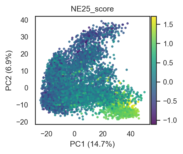
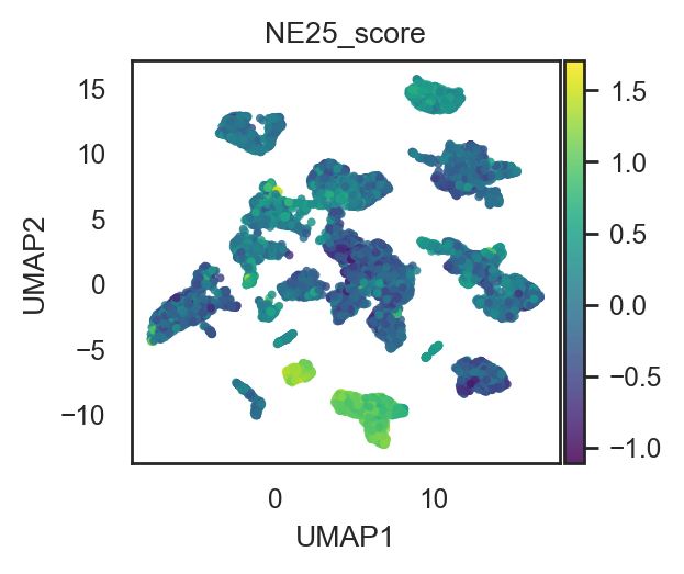
(<Figure size 600x500 with 2 Axes>,
 [<Axes: title={'center': 'NE25_score'}, xlabel='UMAP1', ylabel='UMAP2'>])
6.2.3. Cell cycle status#
This is not very informative in bulk RNAseq data and simply correlates with increased proliferation, but it may be useful to separate specific subgroups of proliferating vs. less proliferating samples in the same tumor type
# Example gene lists (use your preferred human cell-cycle sets)
cell_cycle_genes = {
"s_genes": ["MCM5", "PCNA", "TYMS", "MCM2", "MCM4", "RRM1", "UNG", "GINS2"],
"g2m_genes": ["HMGB2", "CDK1", "NUSAP1", "UBE2C", "BIRC5", "TPX2", "TOP2A"],
}
bk.tl.score_genes_cell_cycle(
    adata,
    s_genes=cell_cycle_genes["s_genes"],
    g2m_genes=cell_cycle_genes["g2m_genes"],
    layer="log1p_cpm",   # or whatever you use for expression scoring
    scale=True,          # optional; often helps if genes have different ranges
)

adata.obs[["S_score", "G2M_score", "phase"]].head()
| S_score | G2M_score | phase | |
|---|---|---|---|
| TCGA-OR-A5JP-01A | 0.489576 | 0.188698 | S |
| TCGA-OR-A5JG-01A | 0.114167 | 0.079497 | S |
| TCGA-OR-A5K1-01A | 0.188504 | -0.089469 | S |
| TCGA-OR-A5JR-01A | -0.190759 | -0.435645 | G1 |
| TCGA-OR-A5KU-01A | -0.556217 | -0.616241 | G1 |
bk.pl.dotplot(adata, var_names=cell_cycle_genes["s_genes"], groupby="Project_ID",
              swap_axes=True,
              dendrogram_top=True,
              dendrogram_rows=True,
              cluster_cols=True,
              cluster_rows=True,
              standard_scale="var",
              colorbar_title=None,
              figsize=(25,3),
              save=DESKTOP + "dotplot_cell_cycle_example.png",
             )
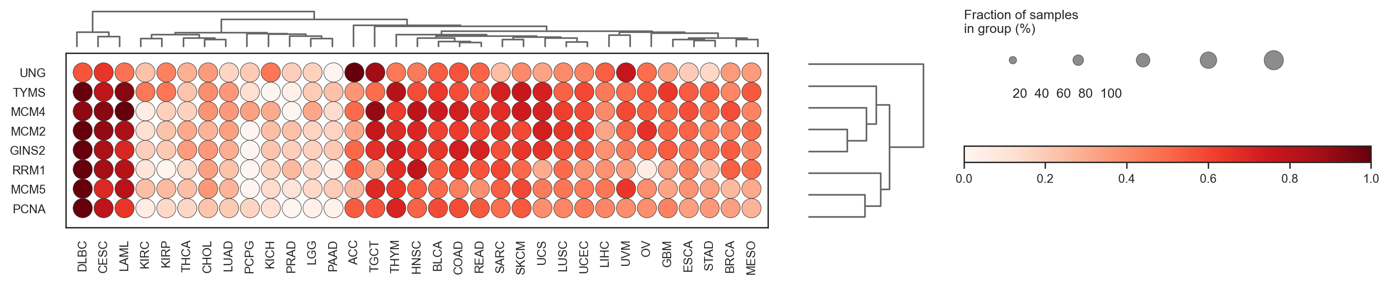
(<Figure size 5000x600 with 5 Axes>, <Axes: >)
cc_names = {
    "S-phase": ["MCM2", "PCNA", "TYMS"],
    "G2/M": ["CDC20", "AURKB", "PLK1"],
}
gene_names = {
    "Proliferation": ["MCM2", "CDC20", "PLK1"],
    "Neuroendocrine": ["ASCL1", "GFAP", "DLL3"],
}
bk.pl.dotplot(adata, var_groups=gene_names, groupby="Project_ID",
              swap_axes=True,
              dendrogram_top=True,
              dendrogram_rows=True,
              cluster_cols=True,
              cluster_rows=True,
              standard_scale="var",
              colorbar_title=None,
              figsize=(18,2),
              save=DESKTOP + "dotplot_example.png",
             )
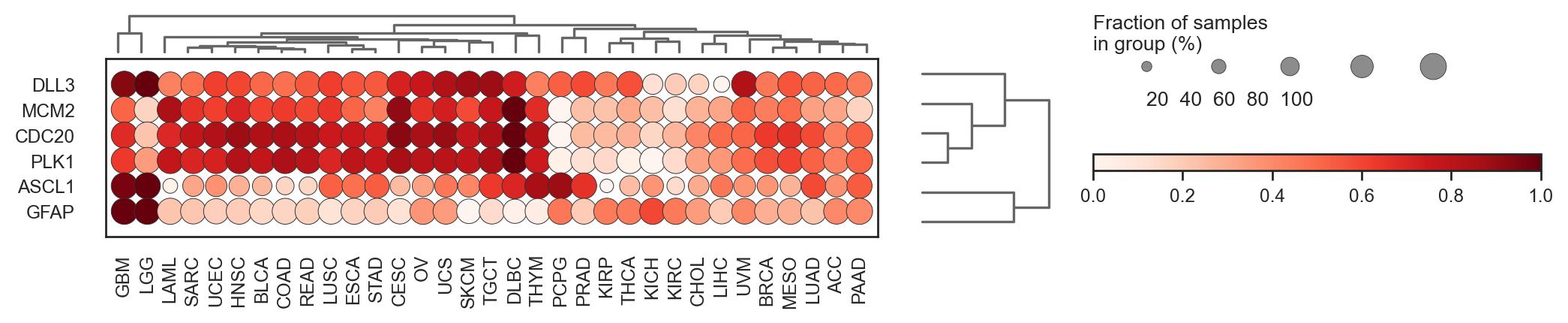
(<Figure size 3600x400 with 5 Axes>, <Axes: >)
bk.pl.pca_scatter(adata, color=["Project_ID", "phase"], figsize=(3,2.5),
                  save=DESKTOP+"PCA_projectID_cellcycle_phase.png", point_size=3,
                 )
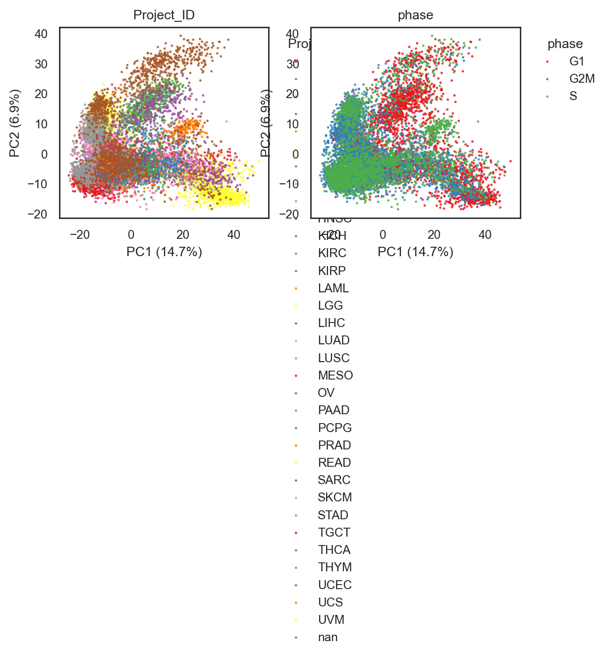
(<Figure size 1200x500 with 2 Axes>,
 array([<Axes: title={'center': 'Project_ID'}, xlabel='PC1 (14.7%)', ylabel='PC2 (6.9%)'>,
        <Axes: title={'center': 'phase'}, xlabel='PC1 (14.7%)', ylabel='PC2 (6.9%)'>],
       dtype=object))
Save .h5ad file with new signatures and gene scores stored in adata.obs
adata.write("../data/h5ad/260127_TCGA_example_in_BULLKpy.h5ad", compression="gzip")
7. Data Exploration#
7.1. General bidimensional representation#
bk.pl.pca_scatter(adata, color=["CDC20", "DLL3"], point_size=2,
          figsize=(3,2.5))
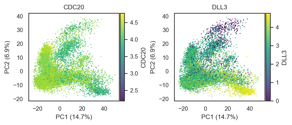
(<Figure size 1200x500 with 4 Axes>,
 array([<Axes: title={'center': 'CDC20'}, xlabel='PC1 (14.7%)', ylabel='PC2 (6.9%)'>,
        <Axes: title={'center': 'DLL3'}, xlabel='PC1 (14.7%)', ylabel='PC2 (6.9%)'>],
       dtype=object))
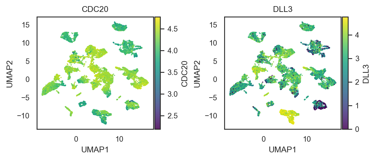
bk.pl.umap(adata, color=["CDC20", "DLL3"], point_size=2,
          figsize=(3,2.5))
(<Figure size 1200x500 with 4 Axes>,
 array([<Axes: title={'center': 'CDC20'}, xlabel='UMAP1', ylabel='UMAP2'>,
        <Axes: title={'center': 'DLL3'}, xlabel='UMAP1', ylabel='UMAP2'>],
       dtype=object))
bk.pl.violin(
    adata,
    keys=["MYC_amplified", "n_genes_detected"],
    groupby="Project_ID",
    #order=["LumA", "LumB", "Her2", "Basal", "Normal"],
    figsize=(12, 3),
    rotate_xticks=90,
    save=DESKTOP + "violin_MYC_qc_genes.png",
)
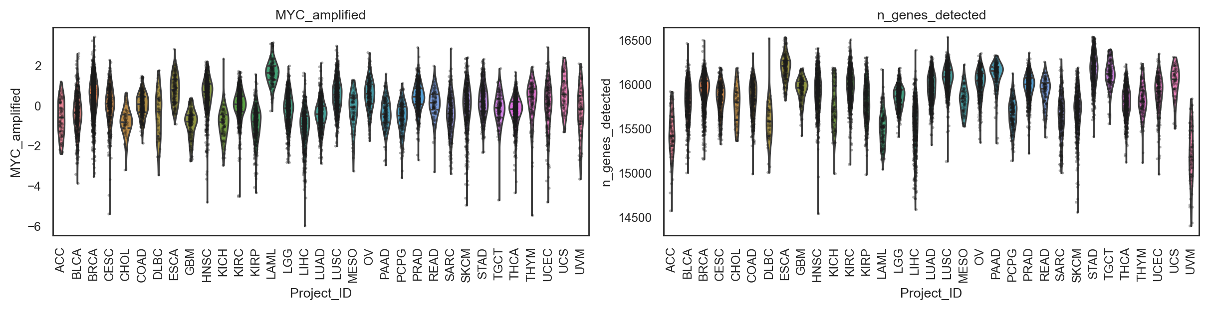
(<Figure size 2400x600 with 2 Axes>,
 array([<Axes: title={'center': 'MYC_amplified'}, xlabel='Project_ID', ylabel='MYC_amplified'>,
        <Axes: title={'center': 'n_genes_detected'}, xlabel='Project_ID', ylabel='n_genes_detected'>],
       dtype=object))
7.2. Select only one/a few categories#
bk.pl.pca_scatter(
    adata,
    color="Project_ID",
    highlight=["LUSC", "LUAD"],
    palette="tab20",
    figsize=(4,2.5),
    save=DESKTOP + "PCA_only_lung_filtered.png",
)
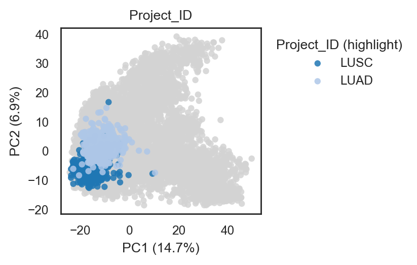
(<Figure size 800x500 with 1 Axes>,
 [<Axes: title={'center': 'Project_ID'}, xlabel='PC1 (14.7%)', ylabel='PC2 (6.9%)'>])
bk.pl.umap(adata, color="Project_ID", point_size=2, highlight=["LUSC", "LUAD"],
          figsize=(4,2.5))
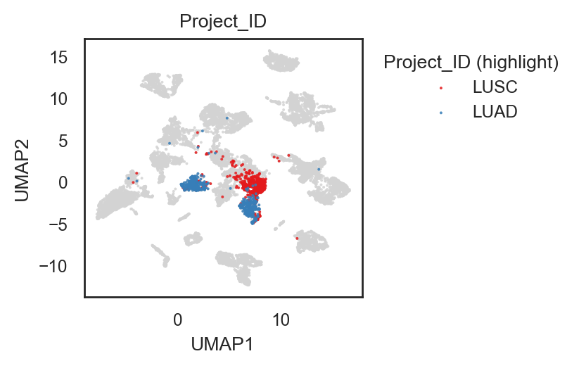
(<Figure size 800x500 with 1 Axes>,
 [<Axes: title={'center': 'Project_ID'}, xlabel='UMAP1', ylabel='UMAP2'>])
bk.pl.pca_scatter(
    adata,
    color=["Project_ID", "DLL3"],
    highlight=["LUSC", "LUAD"],
    palette="tab20",
    figsize=(3,2.5),
)
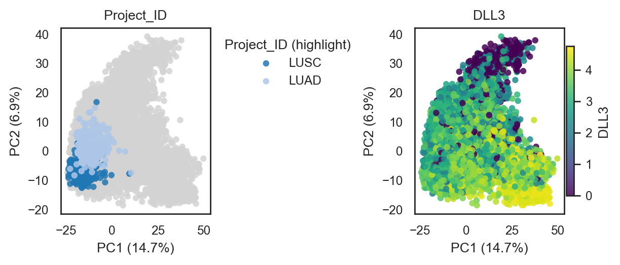
(<Figure size 1200x500 with 3 Axes>,
 array([<Axes: title={'center': 'Project_ID'}, xlabel='PC1 (14.7%)', ylabel='PC2 (6.9%)'>,
        <Axes: title={'center': 'DLL3'}, xlabel='PC1 (14.7%)', ylabel='PC2 (6.9%)'>],
       dtype=object))
7.3. Subfilters#
adata.shape
(11057, 16539)
Define subsets of the large dataset
filter = (adata.obs.Project_ID == "LUAD") | (adata.obs.Project_ID == "LUSC")
adata_lung = adata[filter]
adata_lung.shape
(1108, 16539)
bk.pl.pca_scatter(adata_lung, color=["Project_ID", "DLL3"], palette="tab20",
                  figsize=(3,2.5),
                  save=DESKTOP + "PCA_adata_lung_example.png",
                 )
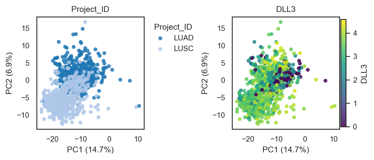
(<Figure size 1200x500 with 3 Axes>,
 array([<Axes: title={'center': 'Project_ID'}, xlabel='PC1 (14.7%)', ylabel='PC2 (6.9%)'>,
        <Axes: title={'center': 'DLL3'}, xlabel='PC1 (14.7%)', ylabel='PC2 (6.9%)'>],
       dtype=object))
bk.pl.violin(
    adata,                                          # complete adata
    keys=["Neuroendocrine_score", "DLL3"],
    groupby="Project_ID",
    order=["LUAD", "LUSC", "BRCA"],                 # but only these groups
    figsize=(3,3),
    rotate_xticks=90,
    save=DESKTOP + "violin_filtered_NE_score_DLL3_lonly_lung.png",
)
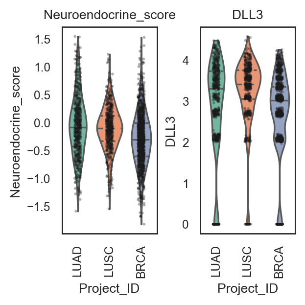
(<Figure size 600x600 with 2 Axes>,
 array([<Axes: title={'center': 'Neuroendocrine_score'}, xlabel='Project_ID', ylabel='Neuroendocrine_score'>,
        <Axes: title={'center': 'DLL3'}, xlabel='Project_ID', ylabel='DLL3'>],
       dtype=object))
bk.pl.violin(
    adata_lung,                                          # only adata_lung
    keys=["Neuroendocrine_score", "DLL3"],
    groupby="Project_ID",
    figsize=(3,3),
    rotate_xticks=90,
    save=DESKTOP + "violin_adata_lung_NE_score_DLL3.png",
)
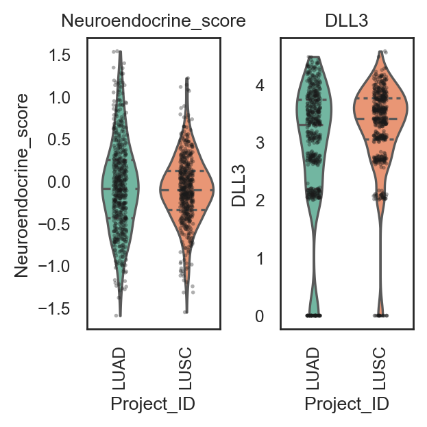
(<Figure size 600x600 with 2 Axes>,
 array([<Axes: title={'center': 'Neuroendocrine_score'}, xlabel='Project_ID', ylabel='Neuroendocrine_score'>,
        <Axes: title={'center': 'DLL3'}, xlabel='Project_ID', ylabel='DLL3'>],
       dtype=object))
bk.pl.dotplot(adata, var_names=["ASCL1","NEUROD1","POU2F3","YAP1"], groupby="Project_ID",
             figsize=(2,5),
             save=DESKTOP + "dotplot_genes_projectID_example.png")
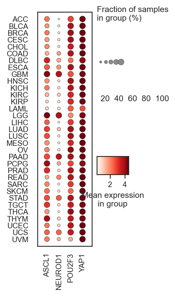
(<Figure size 400x1000 with 3 Axes>, <Axes: >)
bk.pl.umap(adata_lung, color=["Project_ID", "ASCL1", "CDC20"])
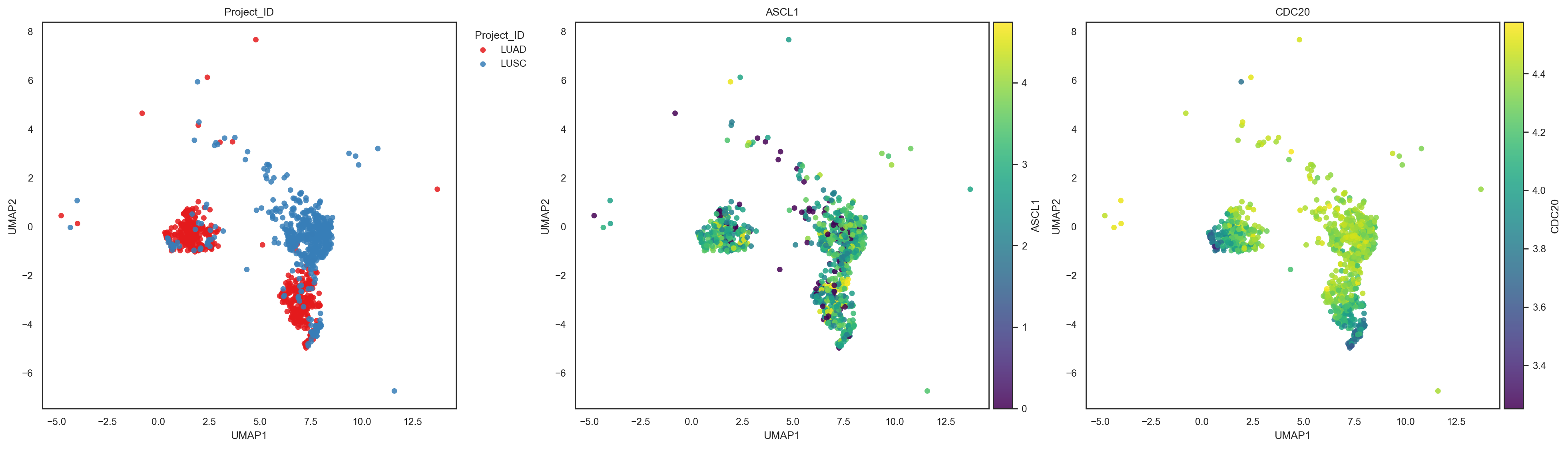
(<Figure size 3900x1100 with 5 Axes>,
 array([<Axes: title={'center': 'Project_ID'}, xlabel='UMAP1', ylabel='UMAP2'>,
        <Axes: title={'center': 'ASCL1'}, xlabel='UMAP1', ylabel='UMAP2'>,
        <Axes: title={'center': 'CDC20'}, xlabel='UMAP1', ylabel='UMAP2'>],
       dtype=object))
Save .h5ad files#
adata.write("../data/h5ad/260127_TCGA_example_in_BULLKpy.h5ad", compression="gzip")
You can also save the lung-specific dataset (or subset later on the large dataset)
adata_lung.write("../data/h5ad/260127_TCGA_LUNG_example_in_BULLKpy.h5ad", compression="gzip")
8. Correlations & Associations#
Recover the stored .h5ad file (if not active in memory)
adata = ad.read_h5ad("../data/h5ad/260127_TCGA_example_in_BULLKpy.h5ad")
adata.shape
(11057, 16539)
Lung cancer samples (n=1108)
filter = (adata.obs.Project_ID == "LUAD") | (adata.obs.Project_ID == "LUSC")
adata_lung = adata[filter]
adata_lung.shape
(1108, 16539)
Lung and breast cancer samples (n=2282)
filter3 = (adata.obs.Project_ID == "LUAD") | (adata.obs.Project_ID == "LUSC") | (adata.obs.Project_ID == "BRCA")
adata_lung_breast = adata[filter3]
adata_lung_breast.shape
(2282, 16539)
8.1. General correlation heatmap#
Correlation between genes (gene expression) or between samples (numeric observations/metadata)
It may be useful as QC (when use="genes") or general correlation between clinical data (use="samples").
cg = bk.pl.corr_heatmap(
    adata_lung_breast,
    use="samples",               # "genes", "samples"
    method="pearson",               # "pearson", "spearman"
    col_colors="Project_ID",
    dendrogram=True,
    remove_cbar_label=True,
    dendrogram_gap=0.08,
    right_margin=1.02,
    cmap="magma",
    figsize=(4,4),
    save=DESKTOP + "corr_heatmap_example_lung_breast.png",
)
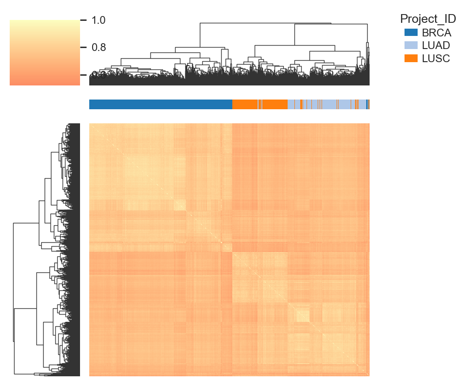
8.2. Correlations between numerical data#
8.2.1. Gene–gene correlations#
# 1) One gene vs ALL genes
df_gene_corr = bk.tl.gene_gene_correlations(
    adata,
    gene="DLL3",
    top_n=50000,
)
df_gene_corr = df_gene_corr.sort_values(by="r", ascending=False)
df_gene_corr.head(3)
| query_gene | gene | r | pval | n | qval | method | batch_key | batch_mode | |
|---|---|---|---|---|---|---|---|---|---|
| 0 | DLL3 | DPF1 | 0.495439 | 0.0 | 11057 | 0.0 | pearson | None | none |
| 1 | DLL3 | GPC2 | 0.472143 | 0.0 | 11057 | 0.0 | pearson | None | none |
| 3 | DLL3 | GAREM2 | 0.455559 | 0.0 | 11057 | 0.0 | pearson | None | none |
df_gene_corr.tail(3)
| query_gene | gene | r | pval | n | qval | method | batch_key | batch_mode | |
|---|---|---|---|---|---|---|---|---|---|
| 13 | DLL3 | RBP5 | -0.420496 | 0.0 | 11057 | 0.0 | pearson | None | none |
| 5 | DLL3 | MAN1A1 | -0.447656 | 0.0 | 11057 | 0.0 | pearson | None | none |
| 2 | DLL3 | CYB5A | -0.463470 | 0.0 | 11057 | 0.0 | pearson | None | none |
# save to an external csv/tsv/excel table
df_gene_corr.to_csv(DESKTOP + "DLL3_gene_correlations.tsv", sep="\t")
plt.figure(figsize=(2.5, 2.5))
sns.scatterplot(y=df.index * (-1), x=df["r"])
plt.show()
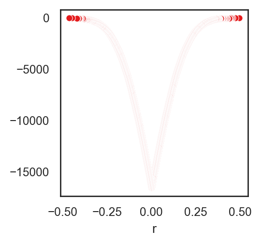
# 2) One gene vs a pathway / gene list

gene_list = ["DLL3", "SOX2", "NEUROD1", "MYCL", "RB1", "MYC", "YAP1"]

df_gene_list_corr = bk.tl.gene_gene_correlations(
    adata,
    gene="ASCL1",
    genes=gene_list,
)
df_gene_list_corr
| query_gene | gene | r | pval | n | qval | method | batch_key | batch_mode | |
|---|---|---|---|---|---|---|---|---|---|
| 0 | ASCL1 | NEUROD1 | 0.312649 | 2.854317e-249 | 11057 | 1.998022e-248 | pearson | None | none |
| 1 | ASCL1 | SOX2 | 0.300498 | 1.639335e-229 | 11057 | 5.737673e-229 | pearson | None | none |
| 2 | ASCL1 | DLL3 | 0.212120 | 1.082448e-112 | 11057 | 2.525712e-112 | pearson | None | none |
| 3 | ASCL1 | MYC | -0.161974 | 7.054600e-66 | 11057 | 1.234555e-65 | pearson | None | none |
| 4 | ASCL1 | RB1 | -0.111084 | 1.059668e-31 | 11057 | 1.483536e-31 | pearson | None | none |
| 5 | ASCL1 | MYCL | 0.053596 | 1.708408e-08 | 11057 | 1.993143e-08 | pearson | None | none |
| 6 | ASCL1 | YAP1 | -0.032775 | 5.671605e-04 | 11057 | 5.671605e-04 | pearson | None | none |
Gene-gene correlation plots
selected_genes = ["PLK1", "CDC20", "DLL3", "GFAP", "NEUROD1", "MKI67", "ASCL1", "ESR1", "CCND1"]
bk.pl.gene_panel_correlation_heatmap(adata, genes=selected_genes,
                                     cluster=True,
                                     figsize=(3,3),
                                     title=" ",
                                     save=DESKTOP + "gene_gene_list_correlation.png",
                                    )
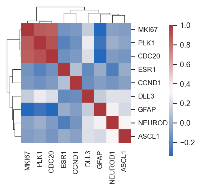
(            MKI67      PLK1     CDC20      ESR1     CCND1      DLL3      GFAP  \
 MKI67    1.000000  0.875672  0.862254 -0.129639 -0.099446  0.137143 -0.337909
 PLK1     0.875672  1.000000  0.910326 -0.213604 -0.141023  0.257718 -0.284913
 CDC20    0.862254  0.910326  1.000000 -0.142390 -0.093755  0.210702 -0.337072
 ESR1    -0.129639 -0.213604 -0.142390  1.000000  0.076438 -0.173379 -0.010453
 CCND1   -0.099446 -0.141023 -0.093755  0.076438  1.000000 -0.150956 -0.080468
 DLL3     0.137143  0.257718  0.210702 -0.173379 -0.150956  1.000000  0.134429
 GFAP    -0.337909 -0.284913 -0.337072 -0.010453 -0.080468  0.134429  1.000000
 NEUROD1 -0.064694 -0.002890 -0.091555 -0.235017 -0.125274  0.220455  0.279339
 ASCL1   -0.083778 -0.052529 -0.119415 -0.011650 -0.070880  0.212120  0.188803

           NEUROD1     ASCL1
 MKI67   -0.064694 -0.083778
 PLK1    -0.002890 -0.052529
 CDC20   -0.091555 -0.119415
 ESR1    -0.235017 -0.011650
 CCND1   -0.125274 -0.070880
 DLL3     0.220455  0.212120
 GFAP     0.279339  0.188803
 NEUROD1  1.000000  0.312649
 ASCL1    0.312649  1.000000  ,
 <Figure size 600x600 with 4 Axes>,
 <seaborn.matrix.ClusterGrid at 0x5d01f7bb0>)
Batch-aware correlation between genes and observations#
# 1) Residualize batch (+ optional covariates) then correlate
df = bk.tl.gene_gene_correlations(
    adata, gene="ASCL1", layer="log1p_cpm",
    batch_key="Batch",                                 # if bactches present
    batch_mode="residualize",
)
# 2) Z-score within each batch, then correlate pooled
df = bk.tl.gene_gene_correlations(
    adata, gene="ASCL1",
    batch_key="Batch", batch_mode="within_batch",
)
# 3) Meta-analyze correlations across batches
df = bk.tl.gene_gene_correlations(
    adata, gene="ASCL1",
    batch_key="Batch", batch_mode="meta",
)
8.2.2. Gene versus Observations Correlations#
# One gene vs all numeric metadata

df_gene_obs_corr = bk.tl.top_gene_obs_correlations(
    adata,
    gene="DLL3",
    layer="log1p_cpm",
    method="spearman",
    top_n=1000,
)
df_gene_obs_corr.head()
| gene | obs | r | pval | n | qval | method | batch_key | batch_mode | |
|---|---|---|---|---|---|---|---|---|---|
| 0 | DLL3 | Neuroendocrine_score | 0.602756 | 0.000000e+00 | 11057 | 0.000000e+00 | spearman | None | none |
| 1 | DLL3 | RETINOL_METABOLISM | -0.424050 | 0.000000e+00 | 9850 | 0.000000e+00 | spearman | None | none |
| 2 | DLL3 | VEGF_PATHWAY | -0.417149 | 0.000000e+00 | 9850 | 0.000000e+00 | spearman | None | none |
| 3 | DLL3 | NE25_score | 0.367105 | 0.000000e+00 | 11057 | 0.000000e+00 | spearman | None | none |
| 4 | DLL3 | RESPONSE_TO_ANDROGEN | 0.356933 | 8.383917e-294 | 9850 | 5.298636e-292 | spearman | None | none |
df_gene_obs_corr = df_gene_obs_corr.sort_values(by="r", ascending=False)
df_gene_obs_corr.head()
| gene | obs | r | pval | n | qval | method | batch_key | batch_mode | |
|---|---|---|---|---|---|---|---|---|---|
| 0 | DLL3 | Neuroendocrine_score | 0.602756 | 0.000000e+00 | 11057 | 0.000000e+00 | spearman | None | none |
| 3 | DLL3 | NE25_score | 0.367105 | 0.000000e+00 | 11057 | 0.000000e+00 | spearman | None | none |
| 4 | DLL3 | RESPONSE_TO_ANDROGEN | 0.356933 | 8.383917e-294 | 9850 | 5.298636e-292 | spearman | None | none |
| 6 | DLL3 | prothrombin_time_result_value | 0.324243 | 3.862038e-02 | 41 | 5.001655e-02 | spearman | None | none |
| 9 | DLL3 | ca_19_9_level | 0.312339 | 5.288786e-02 | 39 | 6.685025e-02 | spearman | None | none |
df_gene_obs_corr.tail()
| gene | obs | r | pval | n | qval | method | batch_key | batch_mode | |
|---|---|---|---|---|---|---|---|---|---|
| 8 | DLL3 | ALK_PATHWAY | -0.317785 | 5.566716e-230 | 9850 | 2.198853e-228 | spearman | None | none |
| 7 | DLL3 | GP7_Estrogen_signaling | -0.318980 | 8.561370e-232 | 9850 | 3.864847e-230 | spearman | None | none |
| 5 | DLL3 | Immune_NSCLC_score | -0.327126 | 2.265228e-244 | 9850 | 1.193020e-242 | spearman | None | none |
| 2 | DLL3 | VEGF_PATHWAY | -0.417149 | 0.000000e+00 | 9850 | 0.000000e+00 | spearman | None | none |
| 1 | DLL3 | RETINOL_METABOLISM | -0.424050 | 0.000000e+00 | 9850 | 0.000000e+00 | spearman | None | none |
# Volcano-style plot
plt.figure(figsize=(2.5, 2.5))
sns.scatterplot(y=df_gene_obs_corr.index*(-1), x=df_gene_obs_corr["r"],)
plt.show()
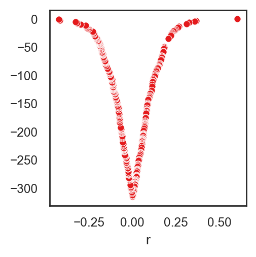
# Volcano-style plot
# This plot gives a problem with pval/qval=0
plt.figure(figsize=(2.5, 2.5))
sns.scatterplot(y=-np.log(df_gene_obs_corr["qval"]), x=df_gene_obs_corr["r"],)
plt.show()
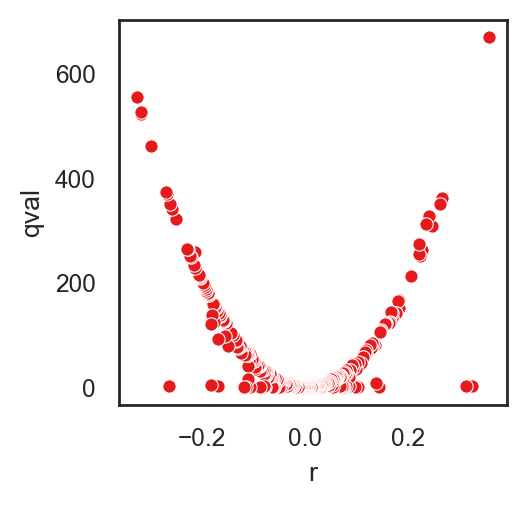
8.2.3. Wide matrix (focus × against) + p/q matrices#
Correlation between numeric values (genes, scores, numeric metadata) and other numeric observations
selected_obs = ["Neuroendocrine_score"]                         # One: "Purity" or several: ["Purity", "TMB"]
obs_list = ["OS.time", "DSS.time", "PFI.time",
            "PFI.time.1", "PFI.time.2", "PFS.time", "DSS.time.cr", "PFI.time.1.cr",
            "PFI.time.2.cr",
            "mitotic_count",
            "Interferon_19272155", "ai1", "lst1", "hrd-loh", "HRD", "S_score",
            "GP2_Immune-Tcell/Bcell", "Leuk", "Stroma", "purity", "ploidy",
            "exposures.cigarettes_per_day", "exposures.pack_years_smoked", "exposures.years_smoked",
            "number_pack_years_smoked", "age_began_smoking_in_years",
            "exposures.alcohol_history", "frequency_of_alcohol_consumption", "amount_of_alcohol_consumption_per_day",
            "amt_alcohol_consumption_per_day",
            "asbestos_exposure_age", "asbestos_exposure_years", "asbestos_exposure_age_last",
           ]

# If necessary:
#adata.obs[obs_list] = adata.obs[obs_list].apply(pd.to_numeric, errors="coerce")
#adata.obs[obs_list] = adata.obs[obs_list].astype(float)          # float, int, "category"
# Ensure they are imported as numeric data
adata.obs[obs_list] = adata.obs[obs_list].apply(pd.to_numeric, errors="coerce")
R, P, Q = bk.tl.obs_obs_corr_matrix(
    adata, focus=selected_obs, against=obs_list, return_p=True, return_q=True,)

res = pd.concat([R, P, Q], keys=["R", "p-val", "q-val"], #names=["source", "row"]
)
res.index = res.index.droplevel(1)
res = res.T.sort_values(by="R", ascending=False)
res
| R | p-val | q-val | |
|---|---|---|---|
| asbestos_exposure_age | 0.656236 | 5.490945e-02 | 9.761679e-02 |
| amt_alcohol_consumption_per_day | 0.213060 | 2.416789e-01 | 3.515329e-01 |
| purity | 0.116548 | 1.232187e-28 | 7.886000e-28 |
| frequency_of_alcohol_consumption | 0.109279 | 3.932324e-02 | 7.402021e-02 |
| S_score | 0.078282 | 1.676213e-16 | 8.939803e-16 |
| exposures.years_smoked | 0.058714 | 1.275284e-01 | 2.040455e-01 |
| ploidy | 0.056437 | 8.239944e-08 | 2.028294e-07 |
| age_began_smoking_in_years | 0.033748 | 5.431162e-01 | 6.951887e-01 |
| lst1 | 0.014942 | 1.559150e-01 | 2.375848e-01 |
| HRD | 0.008915 | 3.972378e-01 | 5.526786e-01 |
| ai1 | 0.004966 | 6.372207e-01 | 7.282522e-01 |
| hrd-loh | 0.004054 | 7.002921e-01 | 7.727361e-01 |
| exposures.pack_years_smoked | 0.003035 | 9.000653e-01 | 9.290997e-01 |
| exposures.cigarettes_per_day | 0.003035 | 9.000653e-01 | 9.290997e-01 |
| number_pack_years_smoked | 0.001192 | 9.606393e-01 | 9.606393e-01 |
| amount_of_alcohol_consumption_per_day | -0.030568 | 5.960948e-01 | 7.075016e-01 |
| OS.time | -0.033450 | 7.920565e-04 | 1.584113e-03 |
| DSS.time.cr | -0.034787 | 5.236978e-04 | 1.117222e-03 |
| DSS.time | -0.034787 | 5.236978e-04 | 1.117222e-03 |
| mitotic_count | -0.055101 | 5.148551e-01 | 6.864734e-01 |
| PFI.time.1.cr | -0.065678 | 5.639919e-11 | 1.503979e-10 |
| PFI.time.1 | -0.065678 | 5.639919e-11 | 1.503979e-10 |
| PFS.time | -0.065889 | 4.894285e-11 | 1.503979e-10 |
| PFI.time | -0.065889 | 4.894285e-11 | 1.503979e-10 |
| PFI.time.2 | -0.073031 | 2.602123e-12 | 1.040849e-11 |
| PFI.time.2.cr | -0.073031 | 2.602123e-12 | 1.040849e-11 |
| Stroma | -0.119430 | 8.298315e-29 | 6.638652e-28 |
| Leuk | -0.123649 | 8.964604e-31 | 9.562245e-30 |
| Interferon_19272155 | -0.134032 | 1.023028e-40 | 1.636845e-39 |
| GP2_Immune-Tcell/Bcell | -0.241616 | 7.739251e-131 | 2.476560e-129 |
| asbestos_exposure_age_last | -0.275681 | 5.969545e-01 | 7.075016e-01 |
| asbestos_exposure_years | -0.528385 | 6.341201e-02 | 1.067992e-01 |
| exposures.alcohol_history | NaN | NaN | NaN |
bk.tl.plot_corr_heatmap(R, title="Correlations", figsize=(7,1),
                       )
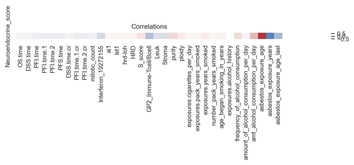
(<Figure size 1400x200 with 2 Axes>, <Axes: title={'center': 'Correlations'}>)
8.2.4. Plot scatter with hue#
bk.pl.corrplot(
    adata,
    x="Neuroendocrine_score",
    y="Proliferation_score",
    color="Project_ID",
    cmap="viridis",
    annotate=False,
    legend=True,
    point_size=5,
    figsize=(2.8,2.5),
    save=DESKTOP + "corr_plot_hue_example.png",
)

(<Figure size 560x500 with 1 Axes>,
 array([<Axes: title={'center': 'Project_ID'}, xlabel='Neuroendocrine_score', ylabel='Proliferation_score'>],
       dtype=object),
 [{'n': 11057,
   'pearson_r': 0.07972541701640834,
   'pearson_p': 4.630208813308786e-17,
   'spearman_rho': 0.11720259467009561,
   'spearman_p': 4.023975448027222e-35,
   'slope': 0.11995563117374855,
   'intercept': 2.4872312516131255e-14}])
bk.pl.corrplot(
    adata_lung,
    x="Neuroendocrine_score",
    y="Proliferation_score",
    color="Project_ID",
    cmap="viridis",
    annotate=False,
    legend=True,
    point_size=5,
    figsize=(3,2.5),
    save=DESKTOP + "corr_plot_hue_example.png",
)
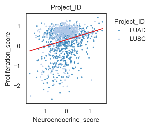
(<Figure size 600x500 with 1 Axes>,
 array([<Axes: title={'center': 'Project_ID'}, xlabel='Neuroendocrine_score', ylabel='Proliferation_score'>],
       dtype=object),
 [{'n': 1108,
   'pearson_r': 0.24213722574867408,
   'pearson_p': 3.0143012236239946e-16,
   'spearman_rho': 0.1885027709202914,
   'spearman_p': 2.543515700986963e-10,
   'slope': 0.3575457239314643,
   'intercept': 0.31669007499857654}])
#Color by gene expression (continuous colormap)
bk.pl.corrplot(
    adata,
    x="Neuroendocrine_score",              # obs
    y="Proliferation_score",               # obs
    color="DLL3",                          # gene in adata.var_names
    layer="log1p_cpm",
    cmap="magma",
    point_size=10,
    annotate=False,
    figsize=(3,2.5),
    save=DESKTOP + "neuro_prolioferation_DLL3.png",
)
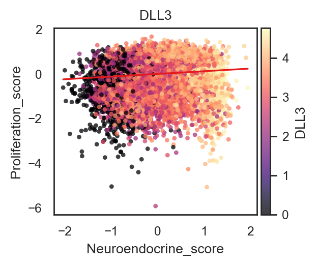
(<Figure size 600x500 with 2 Axes>,
 array([<Axes: title={'center': 'DLL3'}, xlabel='Neuroendocrine_score', ylabel='Proliferation_score'>],
       dtype=object),
 [{'n': 11057,
   'pearson_r': 0.07972541701640834,
   'pearson_p': 4.630208813308786e-17,
   'spearman_rho': 0.11720259467009561,
   'spearman_p': 4.023975448027222e-35,
   'slope': 0.11995563117374855,
   'intercept': 2.4872312516131255e-14}])
#Color by categorical metadata
bk.pl.corrplot(
    adata_lung,
    x="Neuroendocrine_score",
    y="Proliferation_score",
    color="Project_ID",
    palette="tab20",
)
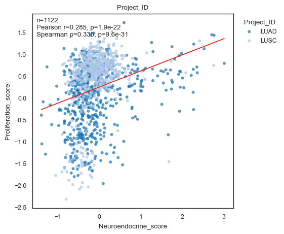
(<Figure size 550x450 with 1 Axes>,
 array([<Axes: title={'center': 'Project_ID'}, xlabel='Neuroendocrine_score', ylabel='Proliferation_score'>],
       dtype=object),
 [{'n': 1122,
   'pearson_r': 0.28523160548334237,
   'pearson_p': 1.905213040533741e-22,
   'spearman_rho': 0.3345589990202715,
   'spearman_p': 9.555423767627166e-31,
   'slope': 0.3686198024643119,
   'intercept': 0.24858805823473168}])
#Color by numerical metadata
bk.pl.corrplot(
    adata_lung,
    x="Neuroendocrine_score",
    y="Proliferation_score",
    color="OS.time",
    cmap="viridis",
)
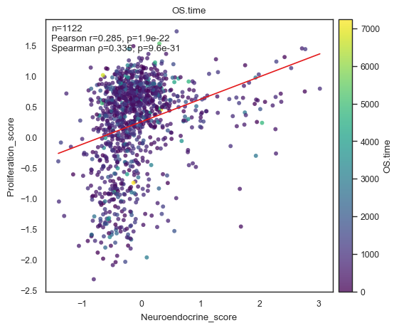
(<Figure size 550x450 with 2 Axes>,
 array([<Axes: title={'center': 'OS.time'}, xlabel='Neuroendocrine_score', ylabel='Proliferation_score'>],
       dtype=object),
 [{'n': 1122,
   'pearson_r': 0.28523160548334237,
   'pearson_p': 1.905213040533741e-22,
   'spearman_rho': 0.3345589990202715,
   'spearman_p': 9.555423767627166e-31,
   'slope': 0.3686198024643119,
   'intercept': 0.24858805823473168}])
bk.tl.plot_corr_scatter(
    adata,
    x="Neuroendocrine_score",
    y="GP2_Immune-Tcell/Bcell",                      # asbestos_exposure_age
    hue="Project_ID",                                 # categorical
    kind="obs_obs",                                  # "gene_obs" or "obs_obs"
    s=10,
    figsize=(3,3),
)
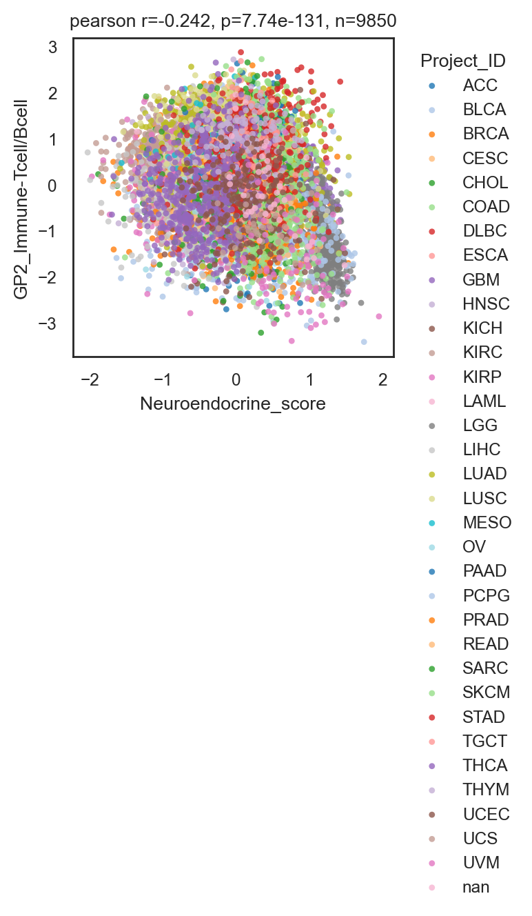
(<Figure size 600x600 with 1 Axes>,
 <Axes: title={'center': 'pearson r=-0.242, p=7.74e-131, n=9850'}, xlabel='Neuroendocrine_score', ylabel='GP2_Immune-Tcell/Bcell'>)
bk.tl.plot_corr_scatter(
    adata_lung_breast,
    x="Neuroendocrine_score",
    y="GP2_Immune-Tcell/Bcell",                      # asbestos_exposure_age
    hue="Project_ID",                                      # categorical
    kind="obs_obs",                                 # "gene_obs" or "obs_obs"
    s=10,
    figsize=(4,3),
)
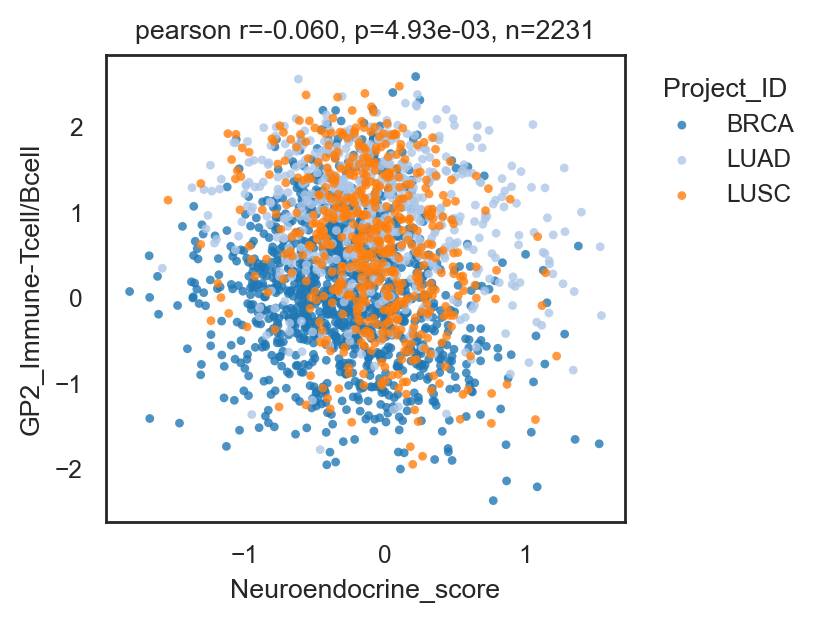
(<Figure size 800x600 with 1 Axes>,
 <Axes: title={'center': 'pearson r=-0.060, p=4.93e-03, n=2231'}, xlabel='Neuroendocrine_score', ylabel='GP2_Immune-Tcell/Bcell'>)
Quick correlations without statistics#
# Numeric obs vs numeric obs (top pairs)

selected_obs = ["Proliferation_score", "Neuroendocrine_score"]                  # single: "purity" or list: ["NE25_score", "purity"]

mat = bk.tl.obs_obs_corr_matrix(adata, focus=selected_obs)
mat.T.sort_values(by=selected_obs, ascending=False)
| Proliferation_score | Neuroendocrine_score | |
|---|---|---|
| score_prolif | 0.966657 | 0.074089 |
| G2M_score | 0.964307 | 0.106292 |
| Module11_Prolif_score | 0.956881 | 0.085962 |
| GP1_Proliferation/DNA_repair | 0.892246 | 0.093708 |
| CASPASE_CASCADE_(APOPTOSIS) | 0.816731 | 0.005034 |
| ... | ... | ... |
| days_to_initial_pathologic_diagnosis | NaN | NaN |
| days_to_definitive_surgical_procedure_performed | NaN | NaN |
| days_to_last_known_alive | NaN | NaN |
| Unnamed: 1061 | NaN | NaN |
| Unnamed: 1062 | NaN | NaN |
333 rows × 2 columns
# Explicit focus × explicit against

focus=["NE25_score", "purity"]
against=["OS.time", "PFI.time", "DSS.time"]

mat = bk.tl.obs_obs_corr_matrix(adata, focus=focus, against=against,)
mat
| OS.time | PFI.time | DSS.time | |
|---|---|---|---|
| NE25_score | -0.004868 | -0.026805 | -0.005169 |
| purity | 0.016129 | -0.006809 | 0.019974 |
mat_first = mat.iloc[:,:20]
mat_first
| OS.time | PFI.time | DSS.time | |
|---|---|---|---|
| NE25_score | -0.004868 | -0.026805 | -0.005169 |
| purity | 0.016129 | -0.006809 | 0.019974 |
fig, ax = plt.subplots(figsize=(12,1))
sns.heatmap(mat_first, cmap="vlag", center=0,
           )
plt.xticks(rotation=45)
plt.show()
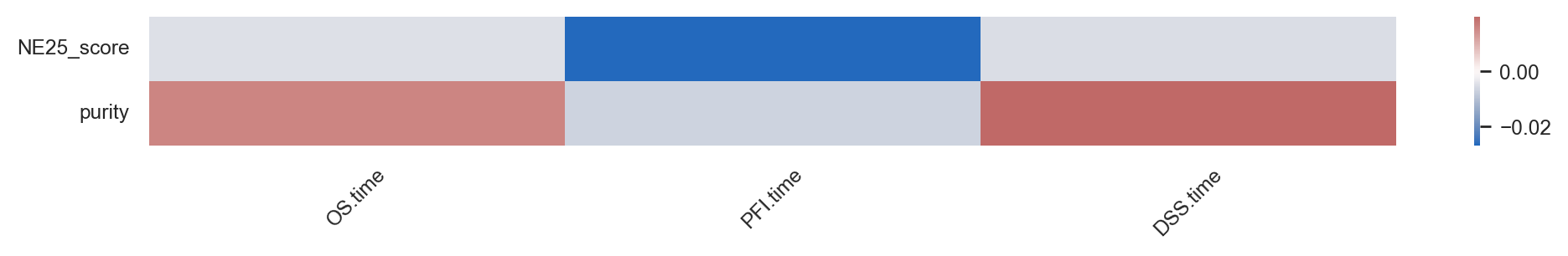
8.3. Associations with categorical data#
Association functions answer a broader statistical question: “Is variable X statistically associated with variable Y?”
They are:
Symmetric (not inherently DE)
Exploratory
Model-light
Often non-parametric
Association functions generalize beyond genes. They work for:
gene ↔ category
numeric obs ↔ category
gene ↔ gene
numeric obs ↔ numeric obs
category ↔ category
They are closer to EDA / statistics than DE.
one single function
Practical advice (bulk RNA-seq)
	•	Prefer Kruskal–Wallis over ANOVA (non-normal)
	•	Always report effect size, not only p-values
	•	For clusters: ARI + Cramér’s V together is ideal
	•	Avoid Pearson with categorical encodings
8.3.1. Gene - categorical (screen genes associated with subtype)#
dfg = bk.tl.gene_categorical_association(
    adata,
    genes=["DLL3", "SOX2", "CDC20"],
    groupby="Project_ID",
    layer="log1p_cpm",
    test="kruskal",                      # "auto", "kruskal", "anova"
    effect_size="epsilon2",              # "auto", "epsilon2", "eta2", "none"
)
dfg
| gene | groupby | n_groups | test | statistic | pval | effect | mean_ACC | mean_BLCA | mean_BRCA | ... | mean_SARC | mean_SKCM | mean_STAD | mean_TGCT | mean_THCA | mean_THYM | mean_UCEC | mean_UCS | mean_UVM | qval | |
|---|---|---|---|---|---|---|---|---|---|---|---|---|---|---|---|---|---|---|---|---|---|
| 0 | DLL3 | Project_ID | 33 | kruskal | 4834.315376 | 0.0 | 0.476090 | 2.850970 | 2.876908 | 2.721556 | ... | 2.809296 | 4.095663 | 2.999894 | 4.110212 | 3.074465 | 2.641142 | 3.217587 | 3.932814 | 3.926824 | 0.0 |
| 1 | SOX2 | Project_ID | 33 | kruskal | 6409.456341 | 0.0 | 0.632245 | 1.709792 | 3.565221 | 2.588665 | ... | 2.444382 | 3.522368 | 3.778907 | 3.643768 | 2.113691 | 3.143804 | 3.077523 | 3.374024 | 2.353429 | 0.0 |
| 2 | CDC20 | Project_ID | 33 | kruskal | 5923.041991 | 0.0 | 0.584023 | 4.068522 | 4.391020 | 4.222561 | ... | 4.340320 | 4.343887 | 4.300291 | 4.391733 | 3.948537 | 4.372171 | 4.382931 | 4.436901 | 4.128115 | 0.0 |
3 rows × 41 columns
columns = ["mean_BRCA", "mean_LUAD", "mean_LUSC"]
#Plot a heatmap of effects:
bk.pl.association_heatmap(
    dfg,
    index="gene",
    columns="groupby",
    values="effect",
    title="Gene-Subtype association (effect size)",
    figsize=(2,2),
    save=DESKTOP + "gene_association_heatmap.png",
)
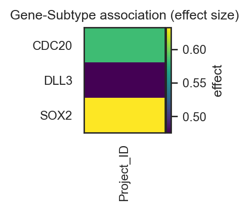
(<Figure size 400x400 with 2 Axes>,
 <Axes: title={'center': 'Gene-Subtype association (effect size)'}>)
bk.pl.gene_association()#
automatic post-hoc (MWU + BH) and bracket annotation
new effect-size aware volcano for categorical associations
bk.pl.gene_association(
    adata_lung,
    gene=["DLL3"],
    groupby="Project_ID",
    layer="log1p_cpm",
    rotate_xticklabels=90,
    annotate_posthoc=True,
    figsize=(2,2.5),
    save=DESKTOP + "gene_association_DLL3_lung.png",
)
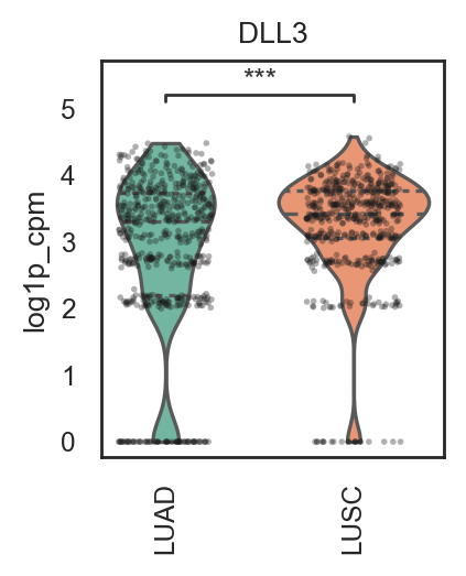
(<Figure size 400x500 with 1 Axes>,
 array([<Axes: title={'center': 'DLL3'}, ylabel='log1p_cpm'>], dtype=object))
bk.pl.gene_association(
    adata_lung,
    gene=["E2F3"],
    groupby="RB1_mut",
    layer="log1p_cpm",
    rotate_xticklabels=90,
    annotate_posthoc=True,
    figsize=(2,2.5),
    save=DESKTOP + "gene_association_E2F3_RB1_mutant.png",
)
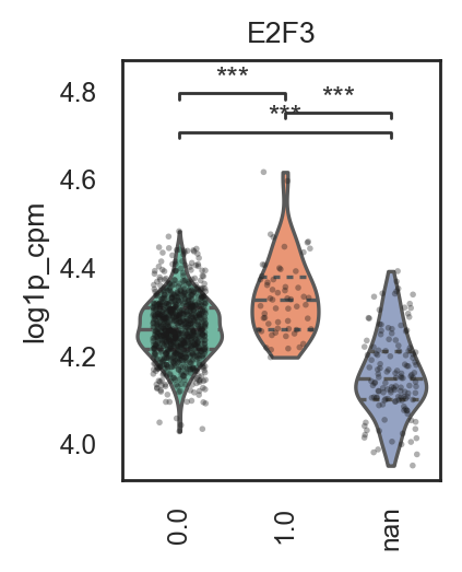
(<Figure size 400x500 with 1 Axes>,
 array([<Axes: title={'center': 'E2F3'}, ylabel='log1p_cpm'>], dtype=object))
# Multiple genes (row of panels)
bk.pl.gene_association(
    adata,
    gene=["DLL3", "CDC20"],
    groupby="Project_ID",
    layer="log1p_cpm",
    rotate_xticklabels=90,
    figsize=(12.0, 3.2),  # per-panel size; total width = 3*4.0
    save=DESKTOP + "associations_DLL3_CDC20_ProjectID.png",
)
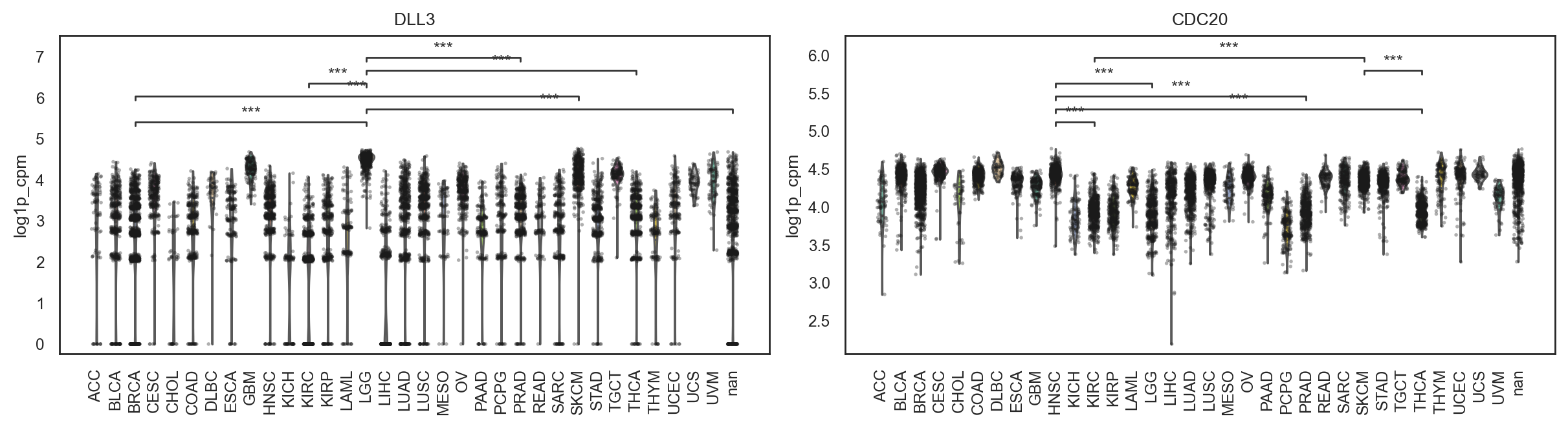
(<Figure size 2400x640 with 2 Axes>,
 array([<Axes: title={'center': 'DLL3'}, ylabel='log1p_cpm'>,
        <Axes: title={'center': 'CDC20'}, ylabel='log1p_cpm'>],
       dtype=object))
fig, ax, df = bk.pl.gene_association_volcano(
    adata,
    groupby="Project_ID",
    group="LUSC",
    reference="LUAD",   # or None for "rest"
    layer="log1p_cpm",
    alpha=0.05,
    figsize=(4,4),
    save=DESKTOP + "assoc_volcano_SCLC_vs_LUAD.png",
)
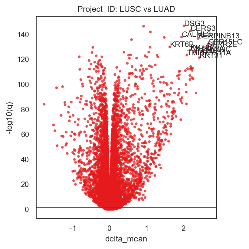
Gene - categorical and rankplots
df = bk.tl.gene_categorical_association(
    adata,
    genes=["RB1", "TP53", "CCND1"],                 # All genes if None. Select one gene or a list of genes
    groupby="Project_ID",
    layer="log1p_cpm",
    test="kruskal",
    effect_size="epsilon2",
)
df
| gene | groupby | n_groups | test | statistic | pval | effect | mean_ACC | mean_BLCA | mean_BRCA | ... | mean_SARC | mean_SKCM | mean_STAD | mean_TGCT | mean_THCA | mean_THYM | mean_UCEC | mean_UCS | mean_UVM | qval | |
|---|---|---|---|---|---|---|---|---|---|---|---|---|---|---|---|---|---|---|---|---|---|
| 0 | RB1 | Project_ID | 33 | kruskal | 2753.242822 | 0.0 | 0.269777 | 4.406087 | 4.329417 | 4.351525 | ... | 4.312524 | 4.399043 | 4.407089 | 4.177166 | 4.372159 | 4.388050 | 4.338921 | 4.299688 | 4.361741 | 0.0 |
| 1 | TP53 | Project_ID | 33 | kruskal | 2246.920817 | 0.0 | 0.219582 | 4.367154 | 4.412832 | 4.393933 | ... | 4.336301 | 4.436881 | 4.376095 | 4.404511 | 4.365795 | 4.457963 | 4.449997 | 4.406609 | 4.546980 | 0.0 |
| 2 | CCND1 | Project_ID | 33 | kruskal | 3443.633392 | 0.0 | 0.338221 | 4.525924 | 4.515059 | 4.566002 | ... | 4.466647 | 4.620286 | 4.502370 | 4.212271 | 4.605875 | 4.465669 | 4.474074 | 4.423103 | 4.708824 | 0.0 |
3 rows × 41 columns
bk.pl.rankplot_association(res=df, gene_col="gene", effect_col="effect", sort_by="qval", n_items=30,
                          figsize=(4,6), save=DESKTOP + "rankplot_association_example.png")
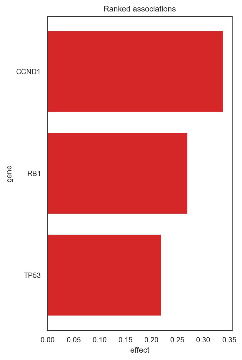
(<Figure size 800x1200 with 1 Axes>,
 <Axes: title={'center': 'Ranked associations'}, xlabel='effect', ylabel='gene'>)
df1 = bk.tl.gene_categorical_association(adata, genes=["DLL3","SOX2"], groupby="Project_ID")
df2 = bk.tl.gene_categorical_association(adata, genes=["DLL3","SOX2"], groupby="Gender")

df_all = pd.concat([df1, df2], ignore_index=True)
df_all
| gene | groupby | n_groups | test | statistic | pval | effect | mean_ACC | mean_BLCA | mean_BRCA | ... | mean_STAD | mean_TGCT | mean_THCA | mean_THYM | mean_UCEC | mean_UCS | mean_UVM | qval | mean_Female | mean_Male | |
|---|---|---|---|---|---|---|---|---|---|---|---|---|---|---|---|---|---|---|---|---|---|
| 0 | DLL3 | Project_ID | 33 | kruskal | 4834.315376 | 0.000000e+00 | 0.476090 | 2.850970 | 2.876908 | 2.721556 | ... | 2.999894 | 4.110212 | 3.074465 | 2.641142 | 3.217587 | 3.932814 | 3.926824 | 0.000000e+00 | NaN | NaN |
| 1 | SOX2 | Project_ID | 33 | kruskal | 6409.456341 | 0.000000e+00 | 0.632245 | 1.709792 | 3.565221 | 2.588665 | ... | 3.778907 | 3.643768 | 2.113691 | 3.143804 | 3.077523 | 3.374024 | 2.353429 | 0.000000e+00 | NaN | NaN |
| 2 | SOX2 | Gender | 2 | kruskal | 173.103740 | 1.553509e-39 | 0.017108 | NaN | NaN | NaN | ... | NaN | NaN | NaN | NaN | NaN | NaN | NaN | 3.107017e-39 | 3.041639 | 3.299033 |
| 3 | DLL3 | Gender | 2 | kruskal | 0.385851 | 5.344882e-01 | -0.000061 | NaN | NaN | NaN | ... | NaN | NaN | NaN | NaN | NaN | NaN | NaN | 5.344882e-01 | 3.043870 | 2.983654 |
4 rows × 43 columns
bk.pl.dotplot_association(df_all, feature_col="gene", groupby_col="groupby", top_n=50,
                         figsize=(2,2))
bk.pl.heatmap_association(df_all, feature_col="gene", groupby_col="groupby", value_col="effect", top_n=40,
                         figsize=(2,2))
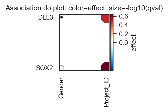
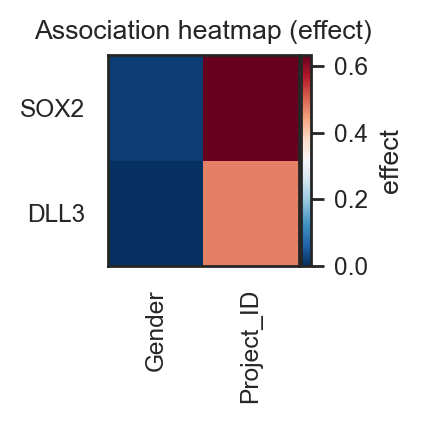
(<Figure size 400x400 with 2 Axes>,
 <Axes: title={'center': 'Association heatmap (effect)'}>)
A) Rank genes associated with a category (associations, not DE)#
res = bk.tl.rank_genes_categorical(
    adata,
    groupby="Project_ID",
    group="LUSC",
    reference="rest",
    layer="log1p_cpm",
    method="mwu",
    store_key="assoc:Project_ID:LUSC_vs_rest",
)
res.head()
| gene | pval | qval | effect_size | mean_group | mean_ref | log2FC | |
|---|---|---|---|---|---|---|---|
| 0 | CTB-11I22.2 | 0.0 | NaN | -0.812866 | 3.160739 | 0.522038 | 2.598035 |
| 1 | RP11-416L21.2 | 0.0 | NaN | -0.705195 | 2.889580 | 0.335939 | 3.104588 |
| 2 | RP11-416L21.1 | 0.0 | NaN | -0.632022 | 1.417213 | 0.130457 | 3.441408 |
| 3 | RP5-1097P24.1 | 0.0 | NaN | -0.512046 | 1.475833 | 0.109945 | 3.746678 |
| 4 | AC128709.3 | 0.0 | NaN | -0.745796 | 3.007364 | 0.384418 | 2.967753 |
B) Volcano plot (effect-size aware)#
bk.pl.volcano_categorical(
    res,
    x="effect_size",   # "effect_size" or x="log2FC"
    q_thr=0.5,
    effect_thr=0.2,
    title="LUSC vs rest (MWU + rank-biserial)",
    #save="figs/volcano_ACC.png",
)
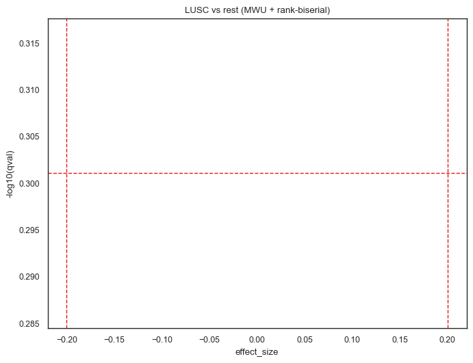
(<Figure size 680x520 with 1 Axes>,
 <Axes: title={'center': 'LUSC vs rest (MWU + rank-biserial)'}, xlabel='effect_size', ylabel='-log10(qval)'>)
D) Automatic posthoc per gene#
posthoc = bk.tl.posthoc_per_gene(
    adata,
    genes=["DLL3", "SOX10", "CDC20"],
    groupby="Project_ID",
    layer="log1p_cpm",
    method="mwu",
)
posthoc["DLL3"].head()
8.3.2. Numeric obs & categorical (which metadata differs across clusters)#
# without statistics
bk.pl.violin(adata, keys=["Neuroendocrine_score"], groupby="Project_ID", figsize=(7,3),
            save=DESKTOP + "violin_groups_example.png"
            )
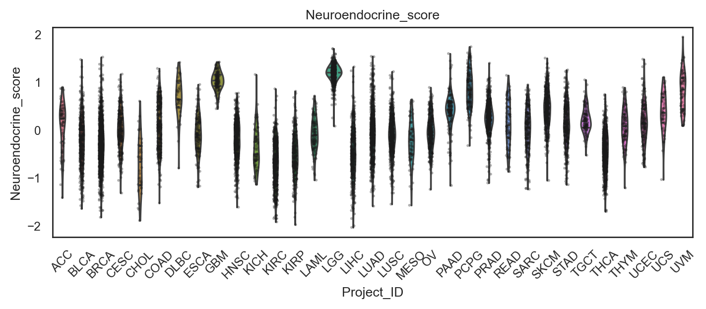
(<Figure size 1400x600 with 1 Axes>,
 array([<Axes: title={'center': 'Neuroendocrine_score'}, xlabel='Project_ID', ylabel='Neuroendocrine_score'>],
       dtype=object))
#Plot one variable with a p-value:
bk.pl.boxplot_with_stats(
    adata,
    y="Neuroendocrine_score",
    groupby="Project_ID",
    kind="violin",                        # "box" or "violin"
    figsize=(5, 2.5),
    save=DESKTOP + "boxplot_stats_example.png",
)
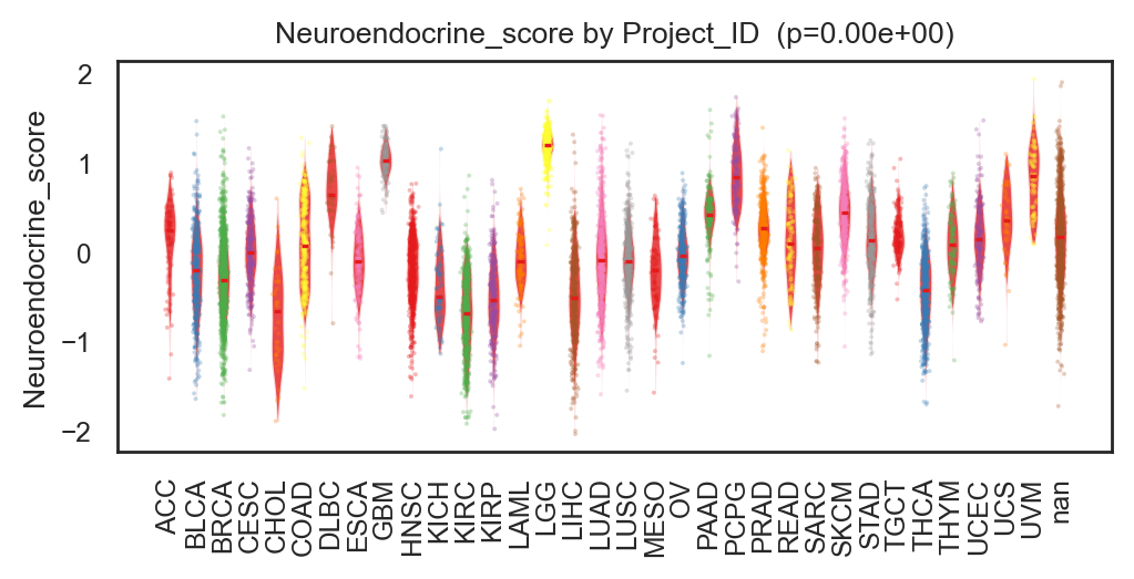
(<Figure size 1000x500 with 1 Axes>,
 <Axes: title={'center': 'Neuroendocrine_score by Project_ID  (p=0.00e+00)'}, ylabel='Neuroendocrine_score'>)
#Plot one variable with a p-value:
bk.pl.boxplot_with_stats(
    adata,
    y="Neuroendocrine_score",
    groupby="RB1_mut",
    kind="box",
    figsize=(2, 2),
    save=DESKTOP + "boxplot_stats_example.png",
)
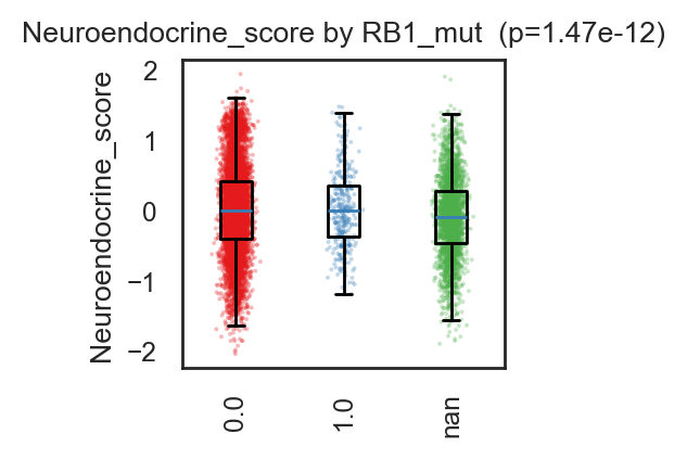
(<Figure size 400x400 with 1 Axes>,
 <Axes: title={'center': 'Neuroendocrine_score by RB1_mut  (p=1.47e-12)'}, ylabel='Neuroendocrine_score'>)
dfo = bk.tl.obs_categorical_association(
    adata,
    obs_keys=["Neuroendocrine_score"],                   # all numeric obs
    groupby="RB1_mut",
    method="kruskal",
)
dfo.head(20)
---------------------------------------------------------------------------
AttributeError                            Traceback (most recent call last)
Cell In[64], line 1
----> 1 dfo = bk.tl.obs_categorical_association(
      2     adata,
      3     obs_keys=["Neuroendocrine_score"],                   # all numeric obs
      4     groupby="RB1_mut",
      5     method="kruskal",
      6 )
      7 dfo.head(20)

AttributeError: module 'bullkpy.tl' has no attribute 'obs_categorical_association'
A) Rank genes associated with a category (associations, not DE)#
# for numeric obs
y = pd.DataFrame({"y": adata.obs["purity"], "grp": adata.obs["Project_ID"]})
post = bk.tl.pairwise_posthoc(y, method="mwu")
post
| group1 | group2 | n1 | n2 | pval | effect | delta_mean | delta_median | qval | |
|---|---|---|---|---|---|---|---|---|---|
| 0 | LUAD | OV | 502 | 407 | 9.646718e-96 | 0.799891 | -0.312945 | -0.360 | 5.093467e-93 |
| 1 | HNSC | OV | 507 | 407 | 9.907419e-82 | 0.736117 | -0.266157 | -0.310 | 2.615558e-79 |
| 2 | KIRC | OV | 495 | 407 | 3.319469e-75 | 0.709180 | -0.224717 | -0.250 | 5.842265e-73 |
| 3 | LGG | LUAD | 511 | 502 | 7.938732e-75 | -0.664294 | 0.251965 | 0.310 | 1.047913e-72 |
| 4 | LUSC | OV | 490 | 407 | 1.232161e-74 | 0.708068 | -0.262391 | -0.310 | 1.301162e-72 |
| ... | ... | ... | ... | ... | ... | ... | ... | ... | ... |
| 523 | GBM | SARC | 152 | 245 | 9.451089e-01 | 0.004135 | 0.016170 | 0.010 | 9.523235e-01 |
| 524 | ACC | KICH | 75 | 66 | 9.521921e-01 | 0.006061 | -0.002412 | -0.005 | 9.576332e-01 |
| 525 | MESO | PRAD | 81 | 471 | 9.750282e-01 | 0.002202 | -0.000010 | 0.030 | 9.783327e-01 |
| 526 | COAD | READ | 282 | 89 | 9.764798e-01 | 0.002112 | -0.005677 | 0.015 | 9.783327e-01 |
| 527 | BRCA | DLBC | 1049 | 46 | 9.954386e-01 | -0.000518 | -0.002160 | 0.035 | 9.954386e-01 |
528 rows × 9 columns
dfo = bk.tl.obs_categorical_association(
    adata,
    groupby="Project_ID",
    obs_keys=["purity", "NE25_score"],
    method="kruskal",
)
dfo
---------------------------------------------------------------------------
AttributeError                            Traceback (most recent call last)
Cell In[36], line 1
----> 1 dfo = bk.tl.obs_categorical_association(
      2     adata,
      3     groupby="Project_ID",
      4     obs_keys=["purity", "NE25_score"],
      5     method="kruskal",
      6 )
      7 dfo

AttributeError: module 'bullkpy.tl' has no attribute 'obs_categorical_association'
bk.pl.rankplot_association(dfo, feature_col="obs", score_col="effect", p_col="qval", top_n=20)
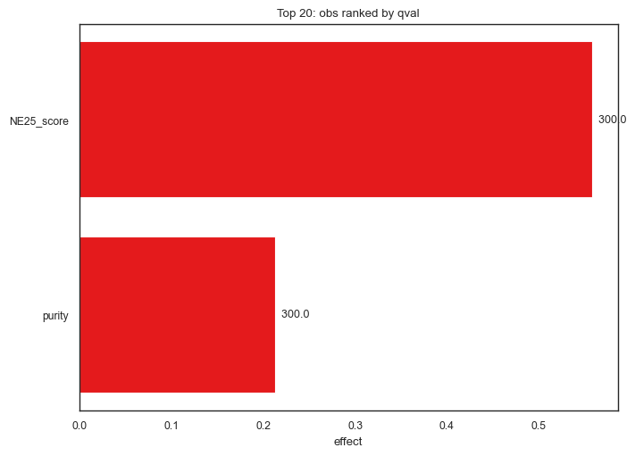
(<Figure size 700x500 with 1 Axes>,
<Axes: title={'center': 'Top 20: obs ranked by qval'}, xlabel='effect'>)
res = bk.tl.rank_genes_categorical(
adata,
groupby="Project_ID",
group="LUSC",
reference="rest",
layer="log1p_cpm",
method="mwu",
store_key="assoc:Project_ID:LUSC_vs_rest",
)
res.head()
| gene | pval | qval | effect_size | mean_group | mean_ref | log2FC | |
|---|---|---|---|---|---|---|---|
| 0 | CTB-11I22.2 | 0.0 | NaN | -0.812866 | 3.160739 | 0.522038 | 2.598035 |
| 1 | RP11-416L21.2 | 0.0 | NaN | -0.705195 | 2.889580 | 0.335939 | 3.104588 |
| 2 | RP11-416L21.1 | 0.0 | NaN | -0.632022 | 1.417213 | 0.130457 | 3.441408 |
| 3 | RP5-1097P24.1 | 0.0 | NaN | -0.512046 | 1.475833 | 0.109945 | 3.746678 |
| 4 | AC128709.3 | 0.0 | NaN | -0.745796 | 3.007364 | 0.384418 | 2.967753 |
8.3.3. Associations between categorical data#
dict_assoc = bk.tl.categorical_association(
adata,
key1="Project_ID", # all numeric obs
key2="RB1_mut",
)
# uses bk.tl.categorical_association()
bk.pl.categorical_confusion(
adata,
key1="Project_ID",
key2="gender",
normalize="row",
cmap="Blues",
figsize=(2,4),
save=DESKTOP + "cat_confusion.png",
)
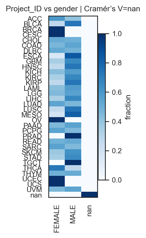
(<Figure size 400x800 with 2 Axes>,
<Axes: title={'center': 'Project_ID vs gender | Cramér’s V=nan'}>)
9. Markers and Differential expression#
9.1. Marker genes#
Which genes are differentially expressed between groups?
Based on Differential expression (DE). Similar to Scanpy rank_genes_groups (group vs rest, etc.)
#rank_genes_groups
9.1.1. Every groups versus the rest#
#Everyone versus the rest
bk.tl.rank_genes_groups(
adata,
groupby="Project_ID",
layer="log1p_cpm",
method="t-test",
n_genes=50,
)
# Get the results for a group
df_lumb = bk.get.rank_genes_groups_df(adata, group="LUAD", sort_by="scores")
df_lumb.head()
| gene | scores | log2FC | pval | qval | mean_group | mean_ref | |
|---|---|---|---|---|---|---|---|
| 0 | SFTPB | 104.414715 | 19.480293 | 0.0 | 0.0 | 16.881305 | 3.378595 |
| 1 | NKX2-1 | 103.835826 | 13.934064 | 0.0 | 0.0 | 11.743011 | 2.084654 |
| 2 | SFTA3 | 98.559444 | 14.346238 | 0.0 | 0.0 | 11.594436 | 1.650381 |
| 3 | SFTA2 | 95.571088 | 12.737869 | 0.0 | 0.0 | 11.479025 | 2.649807 |
| 4 | SLC34A2 | 85.073474 | 12.129740 | 0.0 | 0.0 | 15.283845 | 6.876150 |
# Get the results for all groups
df_all = bk.get.rank_genes_groups_df_all(adata)
df_all.head()
| group | gene | scores | log2FC | pval | qval | mean_group | mean_ref | |
|---|---|---|---|---|---|---|---|---|
| 0 | ACC | STAR | 51.271787 | 18.752414 | 1.671393e-61 | 3.663345e-59 | 16.582610 | 3.584427 |
| 1 | ACC | NR5A1 | 48.126282 | 17.582484 | 2.449793e-59 | 4.956402e-57 | 13.742514 | 1.555265 |
| 2 | ACC | SULT2A1 | 41.167587 | 18.032900 | 1.625689e-54 | 2.689186e-52 | 13.736112 | 1.236658 |
| 3 | ACC | CYP11A1 | 40.627762 | 15.326728 | 6.047854e-54 | 9.728907e-52 | 14.978512 | 4.354833 |
| 4 | ACC | SERPINA5 | 39.269236 | 12.498863 | 2.771207e-54 | 4.541240e-52 | 15.053103 | 6.389551 |
# export
df_all.to_csv(DESKTOP + "rank_genes_groups_all.tsv", sep="\t", index=False)
# Quick table view
bk.pl.rank_genes_groups(adata, n_genes=10, save=DESKTOP + "rank_genes_groups_table.png")

(<Figure size 11060x1060 with 1 Axes>,
<Axes: title={'center': 'Top 10 ranked genes per group'}>)
#3. Dotplot of top markers per group
bk.pl.rank_genes_groups_dotplot(
adata,
groupby="Project_ID",
n_genes=3,
swap_axes=True,
dendrogram_top=True,
#figsize=(4,4),
#save="figs/rank_genes_groups_dotplot.png",
)
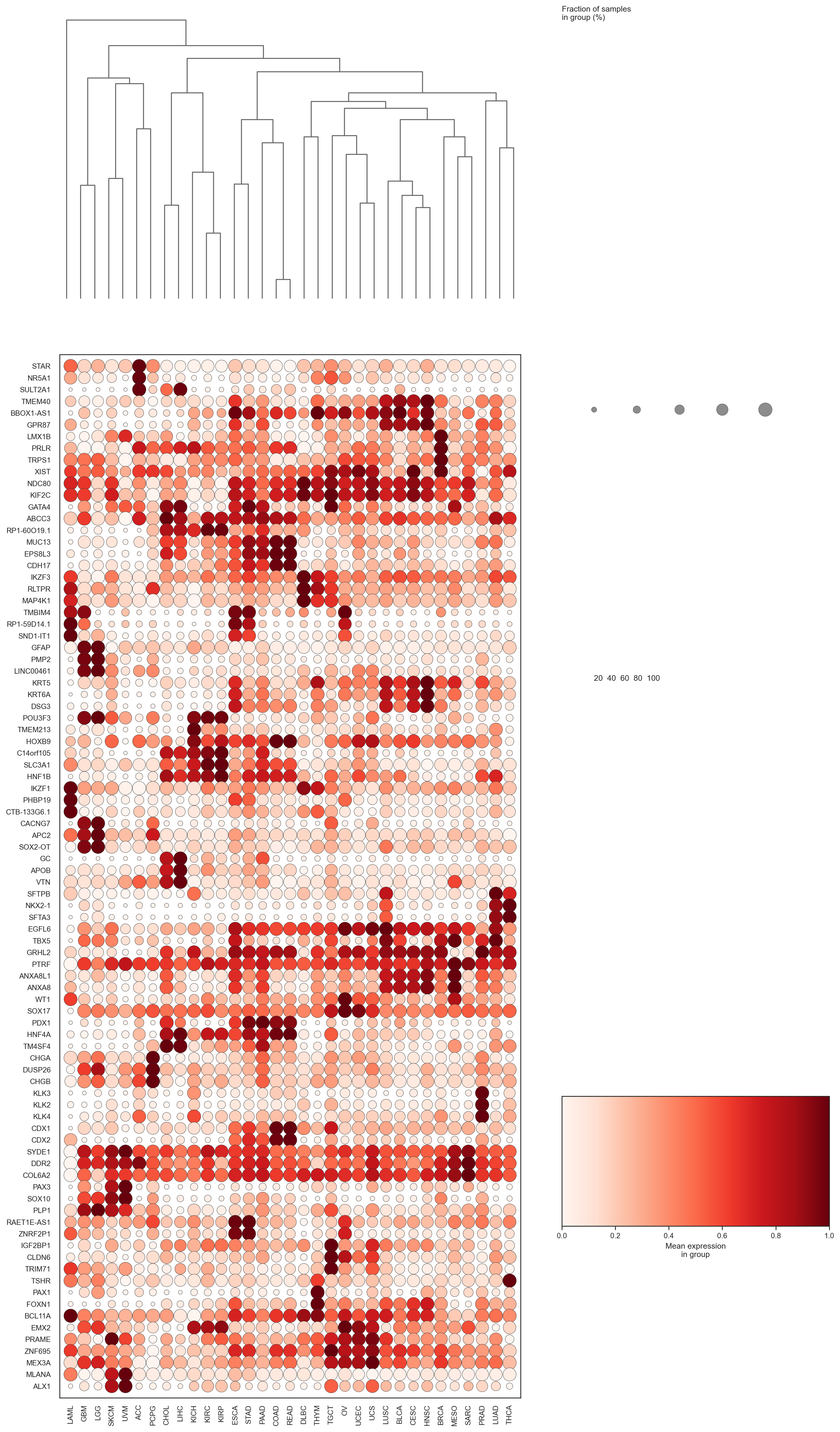
(<Figure size 4020x7912 with 4 Axes>, <Axes: >)
bk.pl.rank_genes_groups_dotplot(
adata,
groupby="Project_ID",
n_genes=3,
swap_axes=True,
dendrogram_top=True,
dendrogram_rows=False,
#save="figs/rank_genes_groups_dotplot.png",
)
(<Figure size 4020x7912 with 4 Axes>, <Axes: >)
#A. Scanpy-like expression dotplot (auto standard_scale=“var”)
bk.pl.rank_genes_groups_dotplot(
adata,
groupby="Project_ID",
n_genes=5,
values_to_plot="expression",
standard_scale="auto",
#save="figs/rgg_dotplot_expression.png",
)
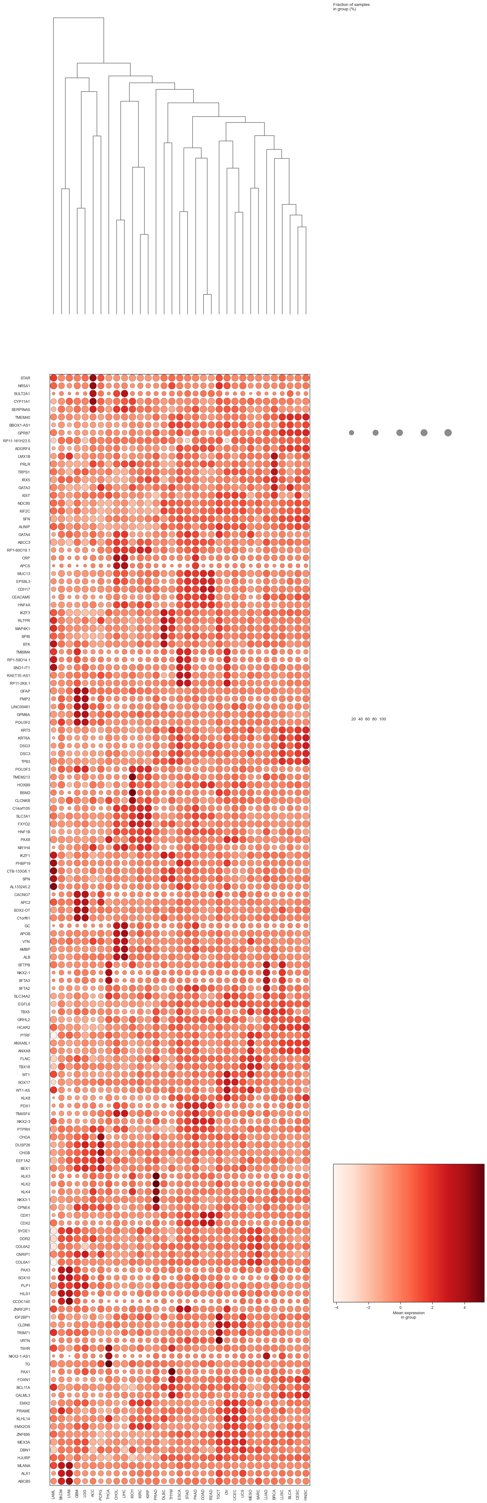
(<Figure size 2155x8010 with 4 Axes>, <Axes: >)
#B. B) Color by log2FC (still sizes by fraction from counts)
bk.pl.rank_genes_groups_dotplot(
adata,
groupby="Project_ID",
n_genes=5,
values_to_plot="logfoldchanges",
min_in_group_fraction=0.05,
max_in_group_fraction=0.95,
#save="figs/rgg_dotplot_logFC.png",
)
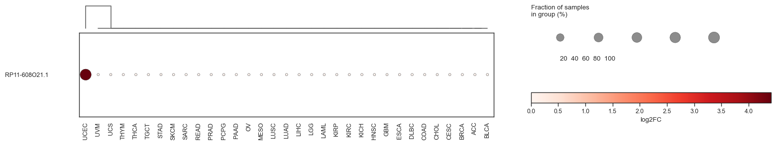
(<Figure size 2155x380 with 4 Axes>, <Axes: >)
9.1.2. One group or a few groups versus other group#
# Group versus specific reference
bk.tl.rank_genes_groups(
adata,
groupby="Project_ID",
groups=["LUAD", "LUSC"],
reference="BRCA",
layer="log1p_cpm",
method="wilcoxon",
n_genes=50,
)
Get the genes from adata.uns['rank_genes_groups'] into a dataframe
df_lumb = bk.get.rank_genes_groups_df(adata, group="LUAD", sort_by="scores")
df_lumb.head()
| gene | scores | log2FC | pval | qval | mean_group | mean_ref | |
|---|---|---|---|---|---|---|---|
| 0 | SFTPB | 34.073980 | 21.689591 | 6.864576e-255 | 1.504572e-251 | 16.881305 | 1.847226 |
| 1 | SFTA3 | 34.066951 | 16.289189 | 7.163340e-302 | 5.383046e-298 | 11.594436 | 0.303630 |
| 2 | NKX2-1 | 34.047337 | 16.410986 | 0.000000e+00 | 0.000000e+00 | 11.743011 | 0.367782 |
| 3 | SFTA2 | 33.987364 | 14.910638 | 3.877076e-258 | 9.711707e-255 | 11.479025 | 1.143758 |
| 4 | HNF1B | 33.916282 | 12.553734 | 2.321304e-261 | 7.182798e-258 | 9.449643 | 0.748057 |
#A. Scanpy-like expression dotplot (auto standard_scale=“var”)
bk.pl.rank_genes_groups_dotplot(
adata,
groupby="Project_ID",
n_genes=5,
values_to_plot="expression",
standard_scale="auto",
#save="figs/rgg_dotplot_expression.png",
)
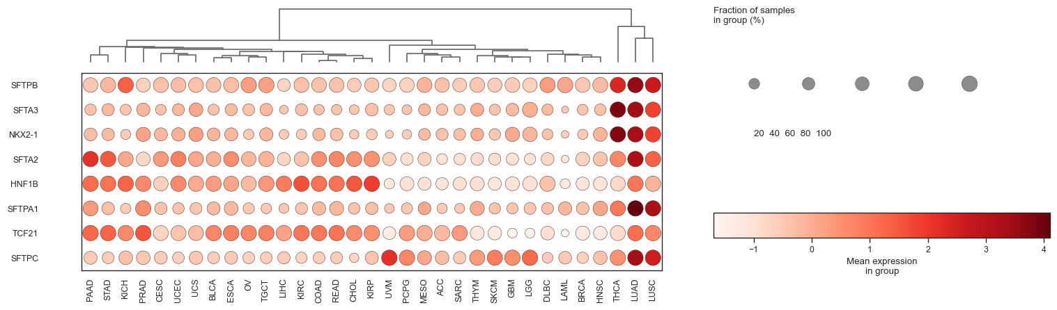
(<Figure size 2155x640 with 4 Axes>, <Axes: >)
9.2. Differential expression#
For bulk RNA-seq, the two most useful layers are:
• a fast exploratory DE (like Scanpy’s “rank genes” idea) → Welch t-test on log1p_cpm
• a proper bulk model → Negative Binomial GLM (DESeq2/edgeR spirit) on raw counts with library-size offset. Important: requires raw counts
Quick best-practice recommendation. Use:
Welch_ttest for fast exploration and ranking
NB GLM only if we either (a) estimate alpha properly, or (b) accept that it’s an approximate baseline
Define comparison#
Select column to select groups from and groups
adata.obs.RB1_mut = adata.obs.RB1_mut.astype("category")
adata.obs.RB1_mut.value_counts()
RB1_mut
0.0 8127
1.0 336
Name: count, dtype: int64
dataset = adata # adata, adata_lung
dataname = "TCGA" # TCGA, TCGA_lung
column = "RB1_mut" # e,g, "Project_ID", "RB1_mut"
groupA = "1.0" # e.g. "LUAD", "1.0"
groupB = "0.0" # e.g. "LUSC", "0.0"
comparison = f"{column}_{groupA}_vs_{groupB}"
comparison
'RB1_mut_1.0_vs_0.0'
dataset = adata_lung # adata, adata_lung
dataname = "TCGA" # TCGA, TCGA_lung
column = "Project_ID" # e,g, "Project_ID", "RB1_mut"
groupA = "LUSC" # e.g. "LUAD", "1.0"
groupB = "LUAD" # e.g. "LUSC", "0.0"
comparison = f"{column}_{groupA}_vs_{groupB}"
comparison
'Project_ID_LUSC_vs_LUAD'
9.2.1. Non-count based, log data: t-test, wilcoxon o welch t-test#
# Fast exploratory (recommended first)
bk.tl.de(adata, groupby=column, group=groupA, reference=groupB,
method="welch_ttest", # wilcoxon ---> explicitly non-count-based
layer_expr="log1p_cpm", # log
)
res = adata.uns["de"][comparison]["results"]
res.head(10)
| gene | log2FC | t | pval | qval | mean_group | mean_ref | |
|---|---|---|---|---|---|---|---|
| 14572 | KRT5 | 9.191601 | 47.521890 | 9.800940e-263 | 5.155588e-258 | 15.743748 | 6.552147 |
| 33474 | DSG3 | 9.411068 | 48.064286 | 1.036572e-251 | 2.726340e-247 | 11.688935 | 2.277868 |
| 48261 | DSC3 | 7.460600 | 44.709548 | 1.774872e-245 | 3.112120e-241 | 12.023859 | 4.563259 |
| 51179 | BNC1 | 6.439554 | 42.130864 | 1.786175e-220 | 2.348954e-216 | 8.997605 | 2.558050 |
| 16752 | CALML3 | 8.876753 | 42.641936 | 8.358320e-220 | 8.793454e-216 | 11.281268 | 2.404515 |
| 39064 | S1PR5 | 3.820233 | 40.410457 | 4.776334e-215 | 4.187492e-211 | 8.542018 | 4.721786 |
| 12836 | CERS3 | 6.834289 | 43.685538 | 2.948562e-207 | 2.215760e-203 | 8.025992 | 1.191702 |
| 47756 | RP11-116G8.5 | 8.010116 | 42.322445 | 3.307243e-203 | 2.174636e-199 | 9.047214 | 1.037098 |
| 8049 | KRT6B | 8.074337 | 38.288022 | 1.569461e-202 | 9.173148e-199 | 11.833138 | 3.758801 |
| 4817 | TP63 | 5.615544 | 38.262135 | 2.993022e-201 | 1.574420e-197 | 12.883407 | 7.267863 |
bk.pl.volcano(res, title="LUSC_vs_LUAD",
alpha=0.4,
top_n_labels = 5, # int
bottom_n_labels = 5,
label_genes = ["RB1", "MYC", "CDK4"], #: Sequence[str] = (),
label_offset=(0.1, 0.8),
p_cutoff = 0.05,
fc_cutoff = 1.0, # optional, set >0 to require |log2FC| >= fc_cutoff
point_size=10,
figsize=(4,3.5),
#save="volcano.png"
)
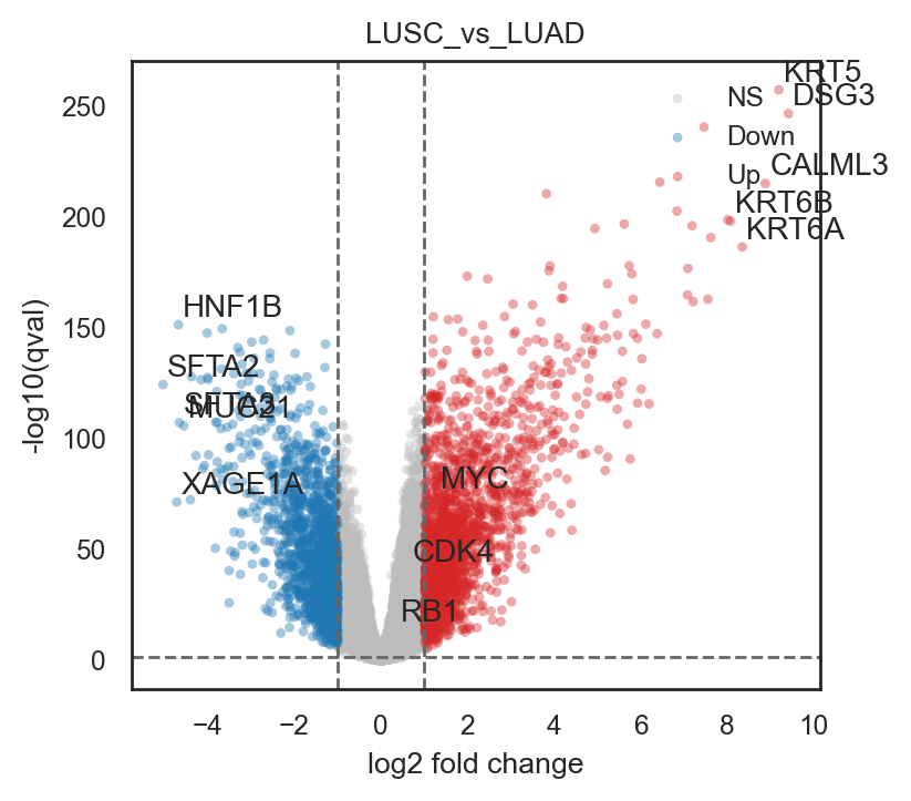
(<Figure size 800x700 with 1 Axes>,
<Axes: title={'center': 'LUSC_vs_LUAD'}, xlabel='log2 fold change', ylabel='-log10(qval)'>)
bk.pl.rankplot(res=res, n_genes=20,
direction="both",
sort_by="qval", # or pval or log2FC
figsize=(4, 3),
) #save="rankplot.png"
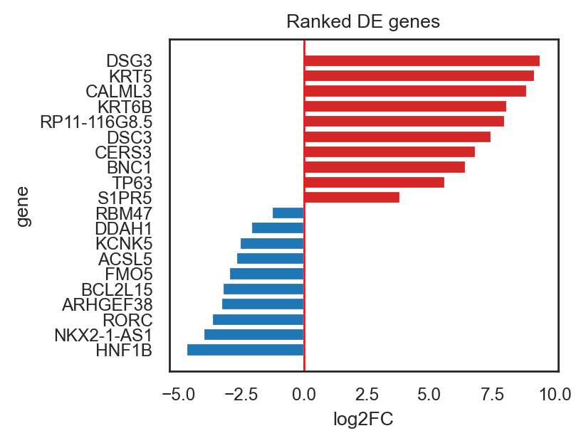
(<Figure size 800x600 with 1 Axes>,
<Axes: title={'center': 'Ranked DE genes'}, xlabel='log2FC', ylabel='gene'>)
bk.pl.ma(
result=res,
mean_col="mean_group",
fc_col="log2FC",
top_n_labels=5,
bottom_n_labels=5,
min_abs_fc = 1.0,
figsize=(5,3),
#label_genes=["DLL3", "SOX10", "CDC20"],
)
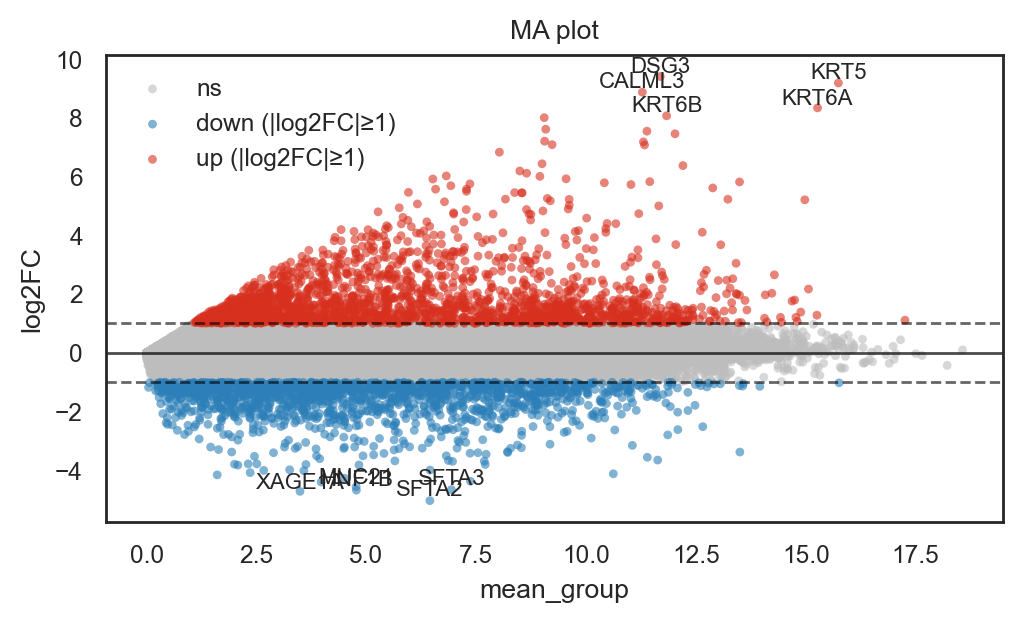
(<Figure size 1000x600 with 1 Axes>,
<Axes: title={'center': 'MA plot'}, xlabel='mean_group', ylabel='log2FC'>)
9.2.2. NB Model (DESeq-like) requires raw counts#
NB Model
This is DESeq2-like, not a full DESeq2 reimplementation:
• DESeq2 does more sophisticated dispersion fitting + shrinkage + outlier handling.
• But for many cohorts, this is already a big leap from “alpha=1”.
# Proper NB model (bulk) --- Requires raw counts
bk.tl.de(
adata,
groupby="Project_ID",
group="LUAD",
reference="LUSC",
method="nb_glm",
#layer_counts="counts",
layer_expr="log1p_cpm",
shrink_dispersion=True,
prior_df=10.0,
)
res = adata.uns["de"]["LUAD_vs_LUSC"]["results"]
res.head(20)
multi-factor DE with a design matrix + contrasts, bulk-style.#
We’ll implement:
• bk.tl.de_glm(…) using NB GLM + DESeq2-like size factors + dispersion (the improved engine),
• supports formulas like ~ Subtype + Batch (and later interactions),
• and a contrast like (“Subtype”, “Basal”, “Luminal”).
This is the bulk equivalent of “design matrix + contrast” from DESeq2/edgeR/limma.
# Make sure covariates are categorical where appropriate
adata.obs["Subtype_PAM50"] = adata.obs["Subtype_PAM50"].astype("category")
adata.obs["Batch"] = adata.obs["Batch"].astype("category") # if you have it
# Run DE adjusted for Batch
bk.tl.de_glm(
adata,
formula="~ Subtype_PAM50 + Batch",
contrast=("Subtype_PAM50", "LumB", "LumA"),
layer_counts="counts",
shrink_dispersion=True,
prior_df=10.0,
)
res = adata.uns["de_glm"]["Subtype_PAM50:LumB_vs_LumA"]["results"]
res.head(25)
# If you don’t have Batch, just:
bk.tl.de_glm(
adata,
formula="~ Subtype_PAM50",
contrast=("Subtype_PAM50", "LumB", "LumA"),
)
res.query("qval < 0.05").head(20)
This initial formula parser supports ~ A + B + C with:
• categorical → dummy-coded (reference = first category)
• numeric → included as-is
No interactions yet (A:B) and no random effects. If you later want patient-paired designs, we’ll add that as a dedicated mode.
If you tell me your typical covariates (Batch, sex, site, patient ID?), I’ll harden the defaults for your use case.
If results are stored in adata.uns[“de_glm”]
10. Pathway and Gene Set Enrichment Analysis#
10.1. GSEA#
# as define above:
print(dataname + "/" + comparison)
TCGA/Project_ID_LUSC_vs_LUAD
GENESETS = "/Users/mmalumbres/Library/CloudStorage/OneDrive-VHIO/BioInformatics/Public_Data/Signatures & GeneSets/GSEA_genesets/2024/"
df_gsea, pre_res = bk.tl.gsea_preranked(
adata,
res=res,
comparison=comparison,
score_col="t", # # good default for preranked
gene_sets=["hallmark"], # ["hallmark", "c2"] also as a list... convenience aliases
#gene_sets=[GENESETS + "h.all.v2024.1.Hs.symbols.gmt"], # if saved locally from MSigDB
#gene_sets=[GENESETS + "h.all.v2024.1.Hs.symbols.gmt", GENESETS + "c2.cp.v2024.1.Hs.symbols.gmt",] # list
outdir="figs/gsea",
return_pre_res=True,
)
# later: concatenate across comparisons
# all_gsea = pd.concat([df_gsea_1, df_gsea_2, ...])
df_gsea.head(3)
| comparison | term | Name | Term | ES | NES | NOM p-val | FDR q-val | FWER p-val | Tag % | Gene % | Lead_genes | |
|---|---|---|---|---|---|---|---|---|---|---|---|---|
| 0 | Project_ID_LUSC_vs_LUAD | 0 | prerank | MSigDB_Hallmark_2020__E2F Targets | 0.801496 | 3.036075 | 0.0 | 0.0 | 0.0 | 151/195 | 12.34% | TFRC;TRA2B;MCM5;RPA1;PHF5A;MCM2;CSE1L;NCAPD2;G... |
| 1 | Project_ID_LUSC_vs_LUAD | 1 | prerank | MSigDB_Hallmark_2020__Myc Targets V1 | 0.779119 | 2.938326 | 0.0 | 0.0 | 0.0 | 149/194 | 15.48% | TRA2B;CNBP;NCBP2;RFC4;MCM5;TCP1;MCM2;FBL;RANBP... |
| 2 | Project_ID_LUSC_vs_LUAD | 2 | prerank | MSigDB_Hallmark_2020__G2-M Checkpoint | 0.776187 | 2.922033 | 0.0 | 0.0 | 0.0 | 143/190 | 12.68% | TRA2B;MCM5;KATNA1;MCM2;UCK2;UBE2S;MYC;CHAF1A;P... |
pre_res.res2d.head(3)
| Name | Term | ES | NES | NOM p-val | FDR q-val | FWER p-val | Tag % | Gene % | Lead_genes | |
|---|---|---|---|---|---|---|---|---|---|---|
| 0 | prerank | MSigDB_Hallmark_2020__E2F Targets | 0.801496 | 3.036075 | 0.0 | 0.0 | 0.0 | 151/195 | 12.34% | TFRC;TRA2B;MCM5;RPA1;PHF5A;MCM2;CSE1L;NCAPD2;G... |
| 1 | prerank | MSigDB_Hallmark_2020__Myc Targets V1 | 0.779119 | 2.938326 | 0.0 | 0.0 | 0.0 | 149/194 | 15.48% | TRA2B;CNBP;NCBP2;RFC4;MCM5;TCP1;MCM2;FBL;RANBP... |
| 2 | prerank | MSigDB_Hallmark_2020__G2-M Checkpoint | 0.776187 | 2.922033 | 0.0 | 0.0 | 0.0 | 143/190 | 12.68% | TRA2B;MCM5;KATNA1;MCM2;UCK2;UBE2S;MYC;CHAF1A;P... |
terms = pre_res.res2d.Term
terms
0 MSigDB_Hallmark_2020__E2F Targets
1 MSigDB_Hallmark_2020__Myc Targets V1
2 MSigDB_Hallmark_2020__G2-M Checkpoint
3 MSigDB_Hallmark_2020__Myc Targets V2
4 MSigDB_Hallmark_2020__mTORC1 Signaling
5 MSigDB_Hallmark_2020__DNA Repair
6 MSigDB_Hallmark_2020__Interferon Alpha Response
7 MSigDB_Hallmark_2020__Mitotic Spindle
8 MSigDB_Hallmark_2020__Interferon Gamma Response
9 MSigDB_Hallmark_2020__Unfolded Protein Response
10 MSigDB_Hallmark_2020__Oxidative Phosphorylation
11 MSigDB_Hallmark_2020__p53 Pathway
12 MSigDB_Hallmark_2020__Coagulation
13 MSigDB_Hallmark_2020__Complement
14 MSigDB_Hallmark_2020__KRAS Signaling Dn
15 MSigDB_Hallmark_2020__Wnt-beta Catenin Signaling
16 MSigDB_Hallmark_2020__Hypoxia
17 MSigDB_Hallmark_2020__KRAS Signaling Up
18 MSigDB_Hallmark_2020__Allograft Rejection
19 MSigDB_Hallmark_2020__UV Response Up
20 MSigDB_Hallmark_2020__PI3K/AKT/mTOR Signaling
21 MSigDB_Hallmark_2020__Estrogen Response Late
22 MSigDB_Hallmark_2020__Spermatogenesis
23 MSigDB_Hallmark_2020__Glycolysis
24 MSigDB_Hallmark_2020__Epithelial Mesenchymal T...
25 MSigDB_Hallmark_2020__Bile Acid Metabolism
26 MSigDB_Hallmark_2020__Apical Junction
27 MSigDB_Hallmark_2020__Apical Surface
28 MSigDB_Hallmark_2020__Cholesterol Homeostasis
29 MSigDB_Hallmark_2020__Inflammatory Response
30 MSigDB_Hallmark_2020__IL-6/JAK/STAT3 Signaling
31 MSigDB_Hallmark_2020__Protein Secretion
32 MSigDB_Hallmark_2020__Xenobiotic Metabolism
33 MSigDB_Hallmark_2020__Reactive Oxygen Species ...
34 MSigDB_Hallmark_2020__TNF-alpha Signaling via ...
35 MSigDB_Hallmark_2020__Estrogen Response Early
36 MSigDB_Hallmark_2020__Hedgehog Signaling
37 MSigDB_Hallmark_2020__heme Metabolism
38 MSigDB_Hallmark_2020__Adipogenesis
39 MSigDB_Hallmark_2020__IL-2/STAT5 Signaling
40 MSigDB_Hallmark_2020__TGF-beta Signaling
41 MSigDB_Hallmark_2020__UV Response Dn
42 MSigDB_Hallmark_2020__Fatty Acid Metabolism
43 MSigDB_Hallmark_2020__Apoptosis
44 MSigDB_Hallmark_2020__Androgen Response
45 MSigDB_Hallmark_2020__Myogenesis
46 MSigDB_Hallmark_2020__Pperoxisome
47 MSigDB_Hallmark_2020__Angiogenesis
48 MSigDB_Hallmark_2020__Notch Signaling
49 MSigDB_Hallmark_2020__Pancreas Beta Cells
Name: Term, dtype: object
ax = pre_res.plot(terms=terms[6], figsize=(6, 6),) # v1.0.5
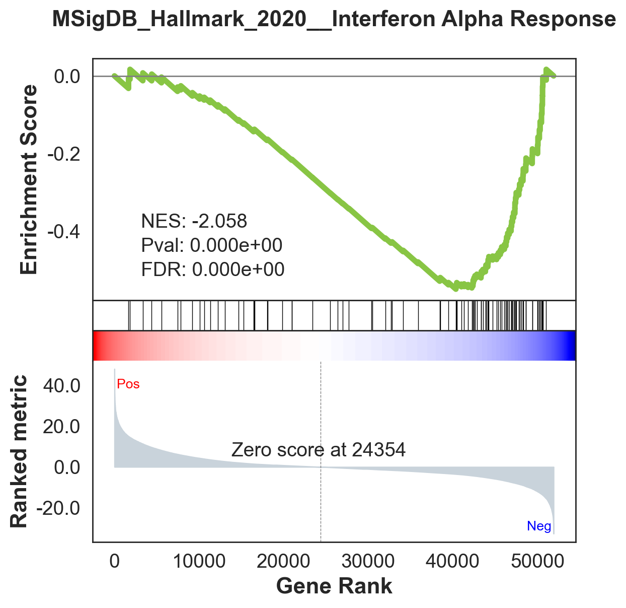
# plot to file
gseaplot(rank_metric=pre_res.ranking, term=terms[0], ofname=DESKTOP + 'your.plot.png', **pre_res.results[terms[0]])
axs = pre_res.plot(terms=terms[0:4],
#legend_kws={'loc': (1.2, 0)}, # set the legend loc
show_ranking=True, # whether to show the second yaxis
figsize=(3,4)
)
# or use this to have more control on the plot
# from gseapy import gseaplot2
# terms = pre_res.res2d.Term[1:5]
# hits = [pre_res.results[t]['hits'] for t in terms]
# runes = [pre_res.results[t]['RES'] for t in terms]
# fig = gseaplot2(terms=terms, ress=runes, hits=hits,
# rank_metric=gs_res.ranking, # rank_metric=pre_res.ranking
# legend_kws={'loc': (1.2, 0)}, # set the legend loc
# figsize=(4,5))
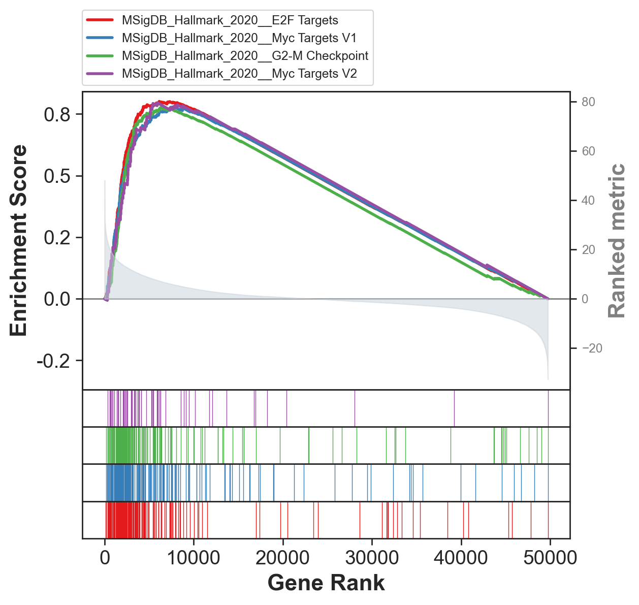
# categorical scatterplot
ax = gspy.dotplot(pre_res.res2d,
column="NOM p-val",
x='Gene_set', # set x axis, so you could do a multi-sample/library comparsion
size=10,
top_term=5,
figsize=(6,6),
title = "Pathways",
xticklabels_rot=45, # rotate xtick labels
show_ring=True, # set to False to revmove outer ring
marker='o',
)
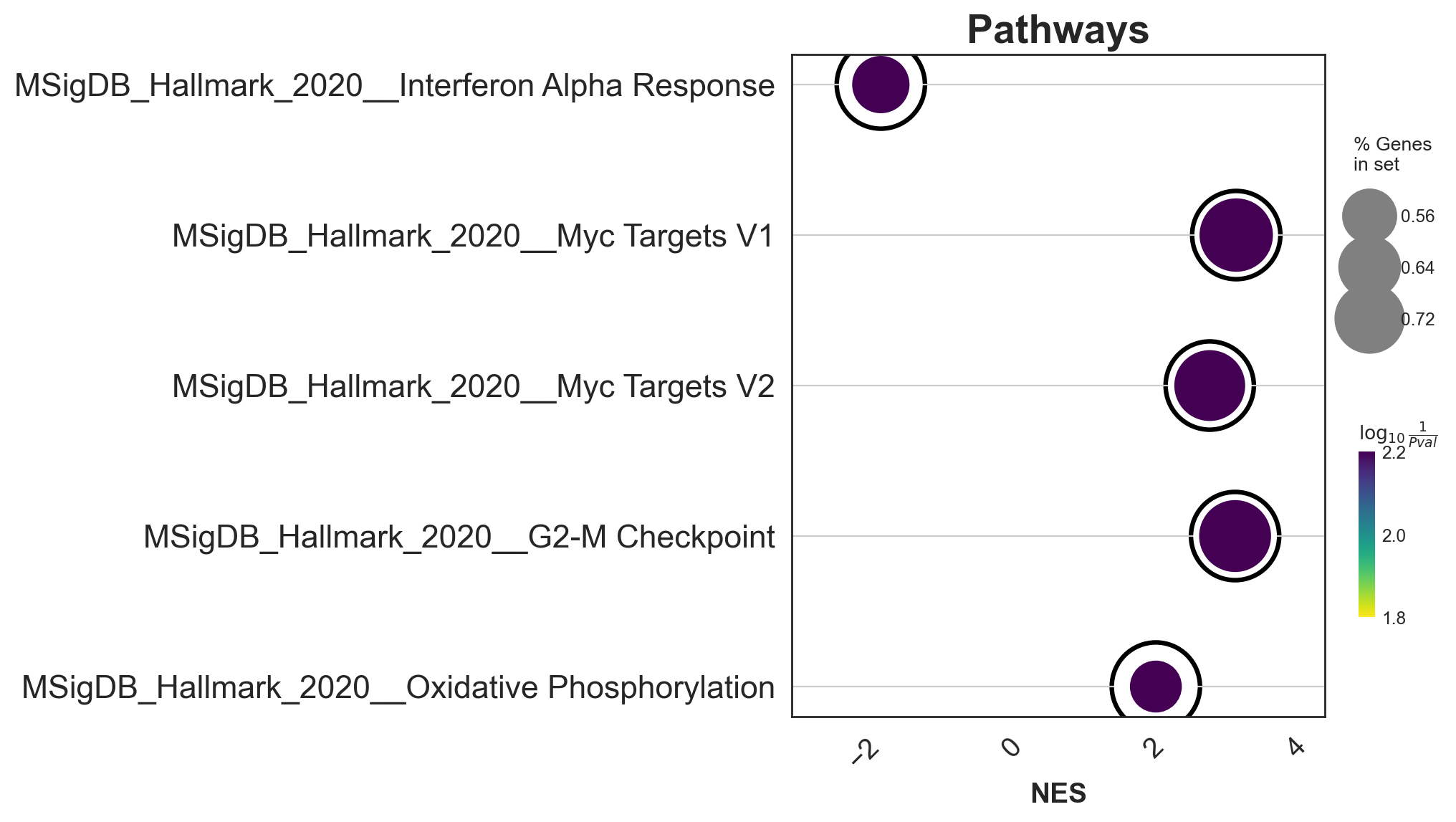
# to save your figure, make sure that ``ofname`` is not None
ax = gspy.dotplot(pre_res.res2d,
column="NOM p-val", #“Adjusted P-value”, “P-value”, “NOM p-val”, “FDR q-val”
title='TEST',
ofname=DESKTOP + "/mix_E3.5_KO_vs_WT.png", # save to file
cmap=plt.cm.viridis,
top_term=12,
size=6, # adjust dot size
figsize=(6,5), cutoff=0.25, show_ring=False)
# to save your figure, make sure that ``ofname`` is not None
ax = gspy.dotplot(pre_res.res2d,
column="FDR q-val",
title='KEGG_2016',
cmap=plt.cm.viridis,
size=6, # adjust dot size
figsize=(4,5), cutoff=0.25, show_ring=False)
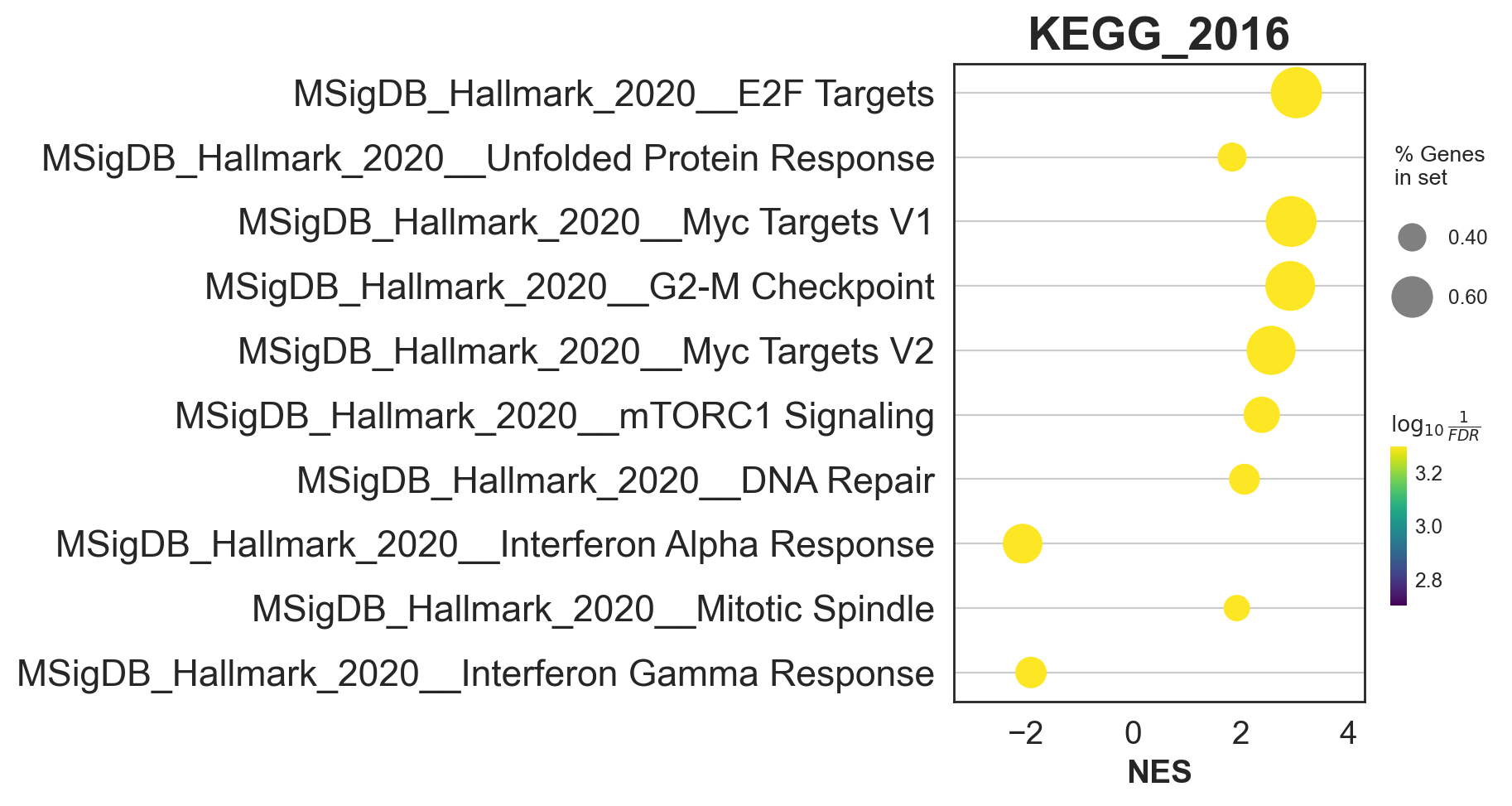
Network Visualization#
# return two dataframe
nodes, edges = enrichment_map(pre_res.res2d)
import networkx as nx
# build graph
G = nx.from_pandas_edgelist(edges,
source='src_idx',
target='targ_idx',
edge_attr=['jaccard_coef', 'overlap_coef', 'overlap_genes'])
fig, ax = plt.subplots(figsize=(8, 8))
# init node cooridnates
pos=nx.layout.spiral_layout(G)
#node_size = nx.get_node_attributes()
# draw node
nx.draw_networkx_nodes(G,
pos=pos,
cmap=plt.cm.RdYlBu_r,
node_color=list(nodes.NES),
node_size=list(nodes.Hits_ratio *1000))
# draw node label
nx.draw_networkx_labels(G,
pos=pos,
labels=nodes.Term.to_dict())
# draw edge
edge_weight = nx.get_edge_attributes(G, 'jaccard_coef').values()
nx.draw_networkx_edges(G,
pos=pos,
width=list(map(lambda x: x*10, edge_weight)),
edge_color='#CDDBD4')
plt.show()
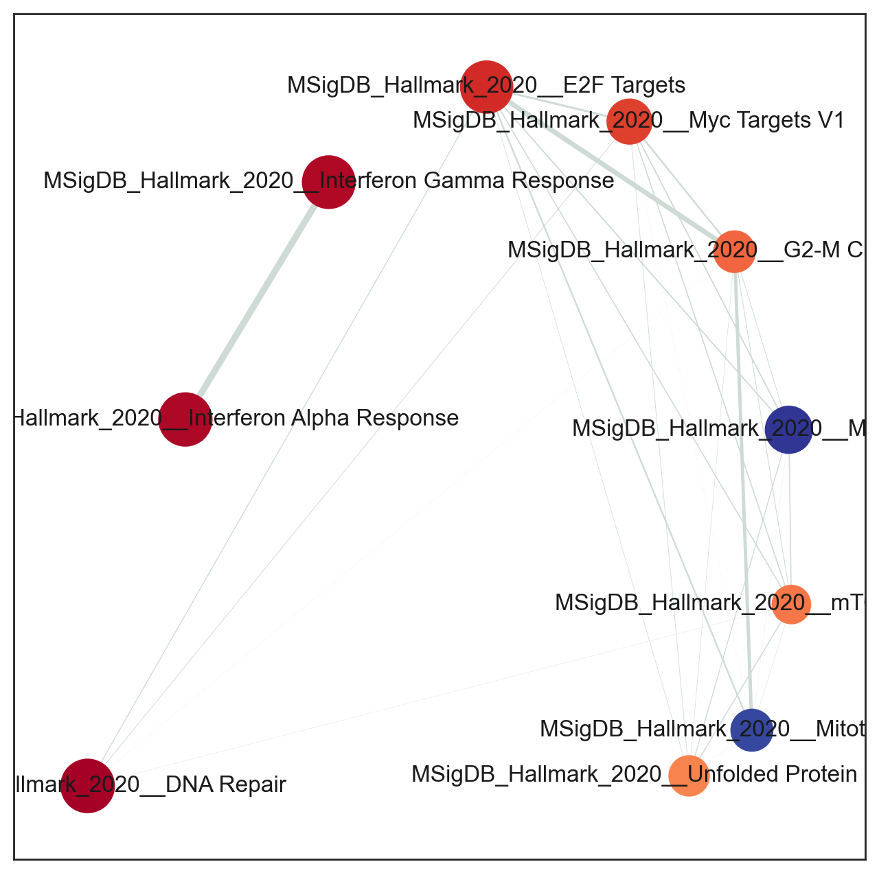
10.2. Leading edge analysis#
i=0
genes = pre_res.res2d.Lead_genes[i].split(";")
genes[:10]
['TFRC',
'TRA2B',
'MCM5',
'RPA1',
'PHF5A',
'MCM2',
'CSE1L',
'NCAPD2',
'GINS3',
'RANBP1']
Expression heatmap of frequent leading-edge genes#
df_expr, g = bk.pl.gsea_leading_edge_heatmap(
adata,
pre_res,
term_idx=slice(0, 30),
use="group_mean",
groupby="Project_ID",
min_gene_freq=3,
max_genes=50,
show_labels=True,
gene_label_fontsize=10.0,
label_fontsize=10.0,
title=None,
show_title=False,
figsize=(8,6),
save=DESKTOP + "leading_edge_expr_heatmap.png",
)
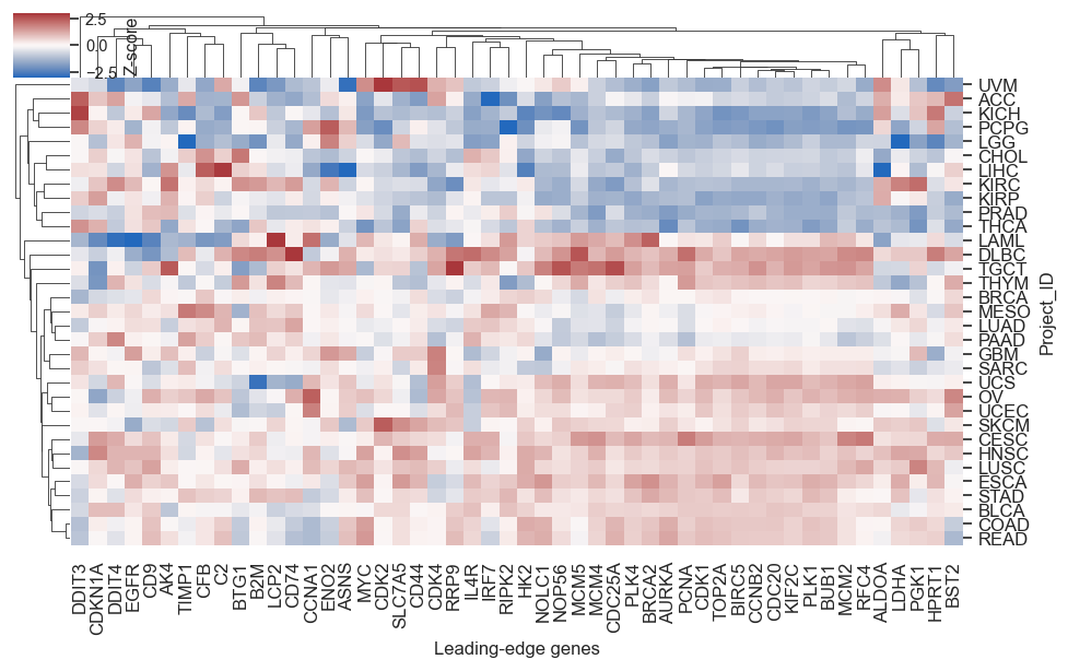
Jaccard similarity between pathways#
dfJ, g = bk.pl.leading_edge_jaccard_heatmap(
pre_res,
term_idx=slice(0, 20),
min_shared_genes=2,
row_cluster=True,
col_cluster=True,
show_title=False,
#ymin=0.3,
figsize=(7,5.5),
save=DESKTOP + "leading_edge_jaccard.png",
)
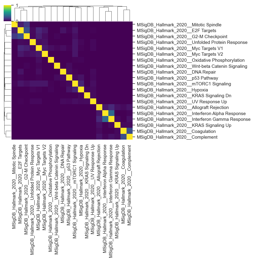
dfJ, gJ = leading_edge_jaccard_heatmap(
pre_res,
term_idx=slice(0, 25), # use only significant pathways (or top N by NES/FDR)
cluster=True,
figsize=(8,8))
plt.savefig("figs/gsea/leading_edge_jaccard.png", dpi=300, bbox_inches="tight")
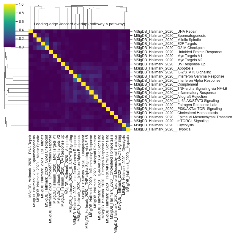
Overlap matrix (pathways × genes) with gene names rotated 90°#
df_le, g = bk.pl.leading_edge_overlap_matrix(
pre_res,
term_idx=slice(0, 15),
min_gene_freq=3,
row_cluster=True,
col_cluster=True,
show_gene_labels=True,
gene_label_fontsize=10,
label_fontsize=10,
show_title=False,
cmap="Reds",
figsize=(12,4),
save=DESKTOP + "leading_edge_overlap.png",
)
# plt.savefig("figs/gsea/leading_edge_overlap.png", dpi=300, bbox_inches="tight")
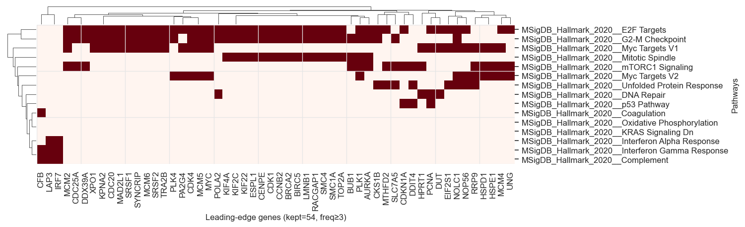
df_le, g = leading_edge_overlap_matrix(
pre_res,
term_idx=slice(0, 30),
min_gene_freq=3, # show only genes shared by >=3 pathways
show_gene_labels=True, # turn on if matrix is small
figsize=(30,8)
)
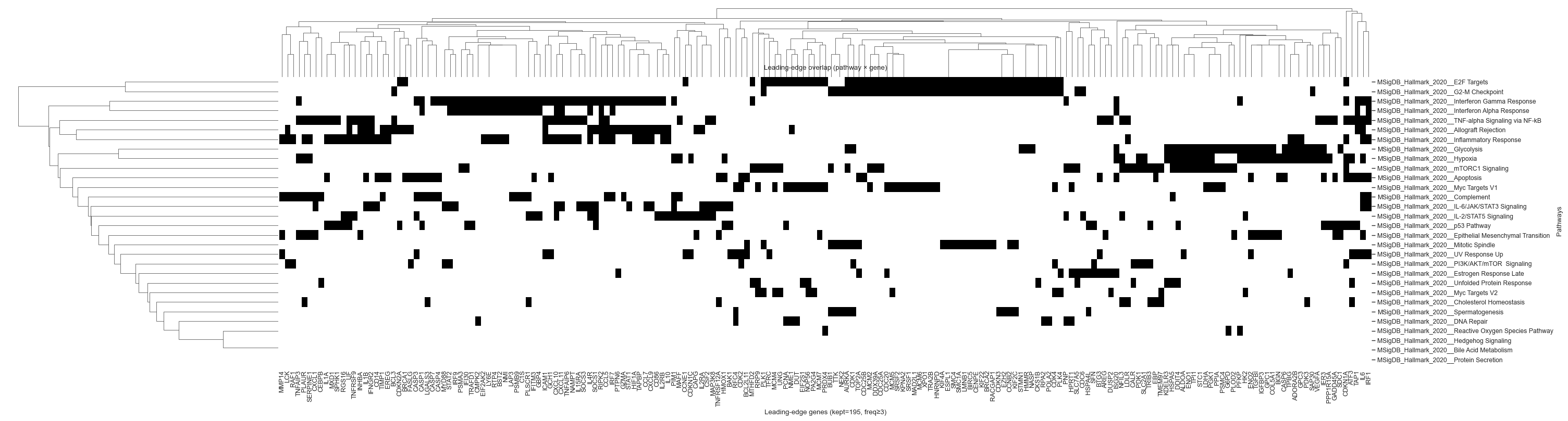
10.3. Gene sets and enrichr#
Enrichr libraries for selected UP- or DOWN-regulated genes (genelists)
res.head(3)
| gene | log2FC | t | pval | qval | mean_group | mean_ref | |
|---|---|---|---|---|---|---|---|
| 14572 | KRT5 | 9.191601 | 47.521890 | 9.800940e-263 | 5.155588e-258 | 15.743748 | 6.552147 |
| 33474 | DSG3 | 9.411068 | 48.064286 | 1.036572e-251 | 2.726340e-247 | 11.688935 | 2.277868 |
| 48261 | DSC3 | 7.460600 | 44.709548 | 1.774872e-245 | 3.112120e-241 | 12.023859 | 4.563259 |
# subset up or down regulated genes
degs_sig = res[res.qval < 0.05]
degs_up = degs_sig[degs_sig.log2FC > 1]
degs_dw = degs_sig[degs_sig.log2FC < -1]
print(degs_up.shape, "UP")
print(degs_dw.shape, "DOWN")
(1943, 7) UP
(1576, 7) DOWN
# Over-representation analysis (Enrichr API)
enr_up = gspy.enrichr(degs_up.gene, # Genelist
gene_sets='GO_Biological_Process_2021', # Geneset
outdir=None)
# dotplot
#UP
gspy.dotplot(enr_up.res2d, figsize=(3,5), title="Up", cmap = plt.cm.autumn_r)
plt.show()
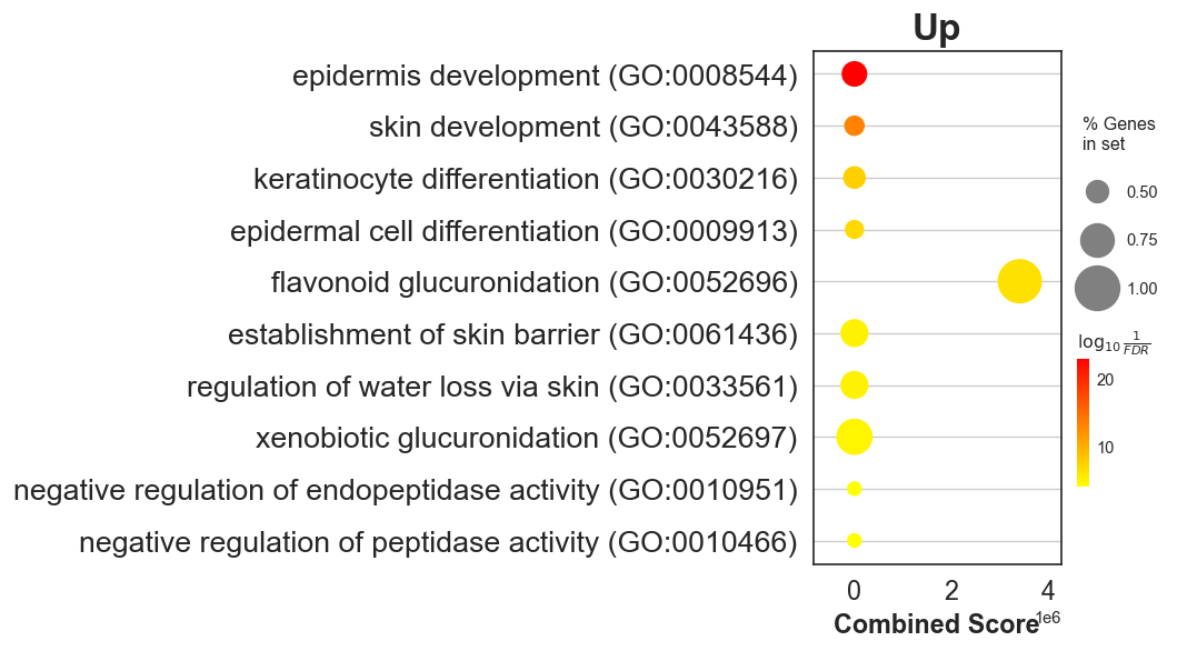
# DOWN
enr_dw = gspy.enrichr(degs_dw.gene,
gene_sets='GO_Biological_Process_2021',
outdir=None)
enr_dw.res2d.Term = enr_dw.res2d.Term.str.split(" \(GO").str[0]
gspy.dotplot(enr_dw.res2d,
figsize=(3,5),
title="Down",
cmap = plt.cm.winter_r,
size=5)
plt.show()
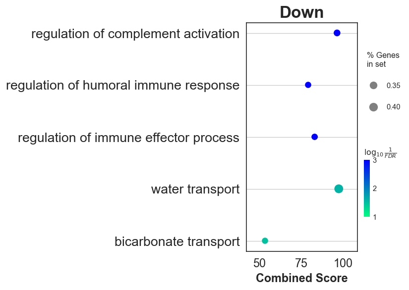
# concat results
enr_up.res2d['UP_DW'] = "UP"
enr_dw.res2d['UP_DW'] = "DOWN"
enr_res = pd.concat([enr_up.res2d.head(), enr_dw.res2d.head()])
enr_res
| Gene_set | Term | Overlap | P-value | Adjusted P-value | Old P-value | Old Adjusted P-value | Odds Ratio | Combined Score | Genes | UP_DW | |
|---|---|---|---|---|---|---|---|---|---|---|---|
| 0 | GO_Biological_Process_2021 | microtubule cytoskeleton organization involved... | 34/128 | 1.549010e-33 | 1.922321e-30 | 0 | 0 | 27.715426 | 2093.836437 | ERCC6L;BUB1B;CDCA8;TTK;WDR62;KIF11;CENPA;SKA1;... | UP |
| 1 | GO_Biological_Process_2021 | mitotic spindle organization (GO:0007052) | 35/157 | 1.342762e-31 | 8.331839e-29 | 0 | 0 | 22.037287 | 1566.529566 | ERCC6L;BUB1B;CDCA8;TTK;WDR62;KIF11;CENPA;SKA1;... | UP |
| 2 | GO_Biological_Process_2021 | mitotic sister chromatid segregation (GO:0000070) | 23/102 | 3.187767e-21 | 1.318673e-18 | 0 | 0 | 21.405822 | 1010.247041 | SPAG5;CDCA5;PLK1;KIF14;CDCA8;NCAPG;KIF23;NCAPH... | UP |
| 3 | GO_Biological_Process_2021 | DNA replication (GO:0006260) | 19/108 | 1.335048e-15 | 4.141987e-13 | 0 | 0 | 15.456652 | 529.387393 | PIF1;FEN1;RMI2;RFC4;DONSON;CDC7;MCM10;CDC6;TIC... | UP |
| 4 | GO_Biological_Process_2021 | sister chromatid segregation (GO:0000819) | 12/34 | 2.838688e-14 | 7.045623e-12 | 0 | 0 | 38.629169 | 1204.953867 | TOP2A;KIF18A;KIF18B;SPAG5;ESPL1;KIFC1;PLK1;CEN... | UP |
| 0 | GO_Biological_Process_2021 | nervous system development | 18/447 | 2.081899e-07 | 2.569064e-04 | 0 | 0 | 4.841409 | 74.484175 | GPM6A;TENM1;RBFOX1;CHRM1;ZBTB16;GFRA1;PCDHA11;... | DOWN |
| 1 | GO_Biological_Process_2021 | central nervous system neuron differentiation | 5/34 | 1.473603e-05 | 6.449331e-03 | 0 | 0 | 18.846447 | 209.670770 | NTRK2;NPY;KNDC1;MAPT;CBLN1 | DOWN |
| 2 | GO_Biological_Process_2021 | membrane depolarization during cardiac muscle ... | 4/17 | 1.567909e-05 | 6.449331e-03 | 0 | 0 | 33.475909 | 370.350098 | ATP1A2;CACNA1D;SCN3B;SCN2B | DOWN |
| 3 | GO_Biological_Process_2021 | chemical synaptic transmission | 12/306 | 3.092587e-05 | 9.540631e-03 | 0 | 0 | 4.578935 | 47.547283 | GABRB3;RIC3;GRIN2A;PTPRN2;CHRM1;GRID1;NPY;GRIK... | DOWN |
| 4 | GO_Biological_Process_2021 | cell differentiation involved in metanephros d... | 3/10 | 9.051690e-05 | 1.422930e-02 | 0 | 0 | 46.386417 | 431.856332 | SALL1;PAX2;POU3F3 | DOWN |
from gseapy.scipalette import SciPalette
sci = SciPalette()
NbDr = sci.create_colormap()
# NbDr
# display multi-datasets
ax = gspy.dotplot(enr_res,figsize=(3,5),
x='UP_DW',
x_order = ["DOWN", "UP"],
title="GO_BP",
cmap = NbDr, # NbDr.reversed()
size=3,
show_ring=True)
ax.set_xlabel("")
plt.show()
---------------------------------------------------------------------------
NameError Traceback (most recent call last)
Cell In[201], line 2
1 # display multi-datasets
----> 2 ax = gspy.dotplot(enr_res,figsize=(3,5),
3 x='UP_DW',
4 x_order = ["DOWN", "UP"],
5 title="GO_BP",
6 cmap = NbDr, # NbDr.reversed()
7 size=3,
8 show_ring=True)
9 ax.set_xlabel("")
10 plt.show()
NameError: name 'enr_res' is not defined
ax = gspy.barplot(enr_res, figsize=(3,5),
group ='UP_DW',
title ="GO_BP",
color = ['b','r'])
---------------------------------------------------------------------------
NameError Traceback (most recent call last)
Cell In[200], line 1
----> 1 ax = gspy.barplot(enr_res, figsize=(3,5),
2 group ='UP_DW',
3 title ="GO_BP",
4 color = ['b','r'])
NameError: name 'enr_res' is not defined
see available libraries: https://maayanlab.cloud/Enrichr/#libraries
TRANSFAC_and_JASPAR_PWMs
TRRUST_Transcription_Factors_2019
ENCODE_and_ChEA_Consensus_TFs_from_ChIP-X
genes_up_list = degs_up["gene"].tolist()
print(len(genes_up_list))
1943
print(len(genes_up_list[:50]))
50
enr_tf = gspy.enrichr(gene_list=genes_up_list[:50],
gene_sets=['TRRUST_Transcription_Factors_2019'],
cutoff=0.1,
organism='Human',
outdir=DESKTOP,
)
enr_tf
<gseapy.enrichr.Enrichr at 0x58a98f9d0>
10.4. Series of parallel comparisons#
dataset = adata # adata, adata_lung
dataname = "TCGA" # TCGA, TCGA_lung
column = "Project_ID" # e,g, "Project_ID", "RB1_mut"
GENESETS = "/Users/mmalumbres/Library/CloudStorage/OneDrive-VHIO/BioInformatics/Public_Data/Signatures & GeneSets/GSEA_genesets/2024/"
adata.obs.Project_ID.unique()
['LGG', 'LIHC', 'CESC', 'LUAD', 'COAD', ..., 'KICH', 'DLBC', NaN, 'ACC', 'CHOL']
Length: 34
Categories (33, object): ['ACC', 'BLCA', 'BRCA', 'CESC', ..., 'THYM', 'UCEC', 'UCS', 'UVM']
# Comparison 1 ---> save to df_gsea1, pre_res1
groupA = "LUAD" # e.g. "LUAD", "1.0"
groupB = "BRCA" # e.g. "LUSC", "0.0"
comparison = f"{column}_{groupA}_vs_{groupB}"
print("Comparison 01...")
bk.tl.de(adata, groupby=column, group=groupA, reference=groupB, method="welch_ttest", layer_expr="log1p_cpm")
res = adata.uns["de"][comparison]["results"]
df_gsea_01, pre_res_01 = bk.tl.gsea_preranked(adata, res=res, comparison=comparison, score_col="t",
gene_sets=["hallmark"], outdir="gsea", return_pre_res=True)
# Comparison 2 ---> save to df_gsea2, , pre_res2
groupA = "LUSC" # e.g. "LUAD", "1.0"
groupB = "BRCA" # e.g. "LUSC", "0.0"
comparison = f"{column}_{groupA}_vs_{groupB}"
print("Comparison 02...")
bk.tl.de(adata, groupby=column, group=groupA, reference=groupB, method="welch_ttest", layer_expr="log1p_cpm")
res = adata.uns["de"][comparison]["results"]
df_gsea_02, pre_res_02 = bk.tl.gsea_preranked(adata, res=res, comparison=comparison, score_col="t",
gene_sets=["hallmark"], outdir="gsea", return_pre_res=True)
print("Merging data from all comparisons...")
# later: concatenate across comparisons
all_gsea = pd.concat([df_gsea_01, df_gsea_02])
all_gsea.head(3)
Comparison 01...
Comparison 02...
Merging data from all comparisons...
| comparison | term | Name | Term | ES | NES | NOM p-val | FDR q-val | FWER p-val | Tag % | Gene % | Lead_genes | |
|---|---|---|---|---|---|---|---|---|---|---|---|---|
| 0 | Project_ID_LUAD_vs_BRCA | 0 | prerank | MSigDB_Hallmark_2020__Allograft Rejection | 0.698233 | 2.557171 | 0.0 | 0.0 | 0.0 | 128/195 | 15.10% | LYN;ICAM1;CCL13;CTSS;ACHE;IL7;C2;SOCS1;IFNAR2;... |
| 1 | Project_ID_LUAD_vs_BRCA | 1 | prerank | MSigDB_Hallmark_2020__Inflammatory Response | 0.697485 | 2.55315 | 0.0 | 0.0 | 0.0 | 121/199 | 14.28% | ROS1;FZD5;ICAM4;LYN;ICAM1;CCL20;SLC4A4;LAMP3;C... |
| 2 | Project_ID_LUAD_vs_BRCA | 2 | prerank | MSigDB_Hallmark_2020__Interferon Gamma Response | 0.658335 | 2.445876 | 0.0 | 0.0 | 0.0 | 98/198 | 12.50% | UPP1;ICAM1;METTL7B;PTGS2;ST3GAL5;BANK1;CASP4;P... |
all_gsea
| comparison | term | Name | Term | ES | NES | NOM p-val | FDR q-val | FWER p-val | Tag % | Gene % | Lead_genes | |
|---|---|---|---|---|---|---|---|---|---|---|---|---|
| 0 | Project_ID_LUAD_vs_BRCA | 0 | prerank | MSigDB_Hallmark_2020__Allograft Rejection | 0.698233 | 2.557171 | 0.0 | 0.0 | 0.0 | 128/195 | 15.10% | LYN;ICAM1;CCL13;CTSS;ACHE;IL7;C2;SOCS1;IFNAR2;... |
| 1 | Project_ID_LUAD_vs_BRCA | 1 | prerank | MSigDB_Hallmark_2020__Inflammatory Response | 0.697485 | 2.55315 | 0.0 | 0.0 | 0.0 | 121/199 | 14.28% | ROS1;FZD5;ICAM4;LYN;ICAM1;CCL20;SLC4A4;LAMP3;C... |
| 2 | Project_ID_LUAD_vs_BRCA | 2 | prerank | MSigDB_Hallmark_2020__Interferon Gamma Response | 0.658335 | 2.445876 | 0.0 | 0.0 | 0.0 | 98/198 | 12.50% | UPP1;ICAM1;METTL7B;PTGS2;ST3GAL5;BANK1;CASP4;P... |
| 3 | Project_ID_LUAD_vs_BRCA | 3 | prerank | MSigDB_Hallmark_2020__TNF-alpha Signaling via ... | 0.639815 | 2.383453 | 0.0 | 0.0 | 0.0 | 112/198 | 14.73% | CXCL3;CSF2;ICAM1;CCL20;CXCL1;BMP2;CXCL2;PTGS2;... |
| 4 | Project_ID_LUAD_vs_BRCA | 4 | prerank | MSigDB_Hallmark_2020__IL-6/JAK/STAT3 Signaling | 0.715757 | 2.371309 | 0.0 | 0.0 | 0.0 | 55/87 | 14.08% | CXCL3;CSF2;CXCL1;TNFRSF21;CD38;OSMR;IL7;SOCS1;... |
| ... | ... | ... | ... | ... | ... | ... | ... | ... | ... | ... | ... | ... |
| 45 | Project_ID_LUSC_vs_BRCA | 45 | prerank | MSigDB_Hallmark_2020__Oxidative Phosphorylation | 0.312852 | 1.154602 | 0.1376 | 0.17681 | 0.988 | 69/184 | 19.15% | LDHB;POR;SLC25A5;FDX1;BAX;TOMM22;POLR2F;SDHD;E... |
| 46 | Project_ID_LUSC_vs_BRCA | 46 | prerank | MSigDB_Hallmark_2020__Spermatogenesis | 0.316611 | 1.122745 | 0.220367 | 0.219801 | 0.996 | 46/133 | 17.29% | CFTR;DCC;NOS1;POMC;GFI1;DMRT1;TLE4;PGS1;RFC4;G... |
| 47 | Project_ID_LUSC_vs_BRCA | 47 | prerank | MSigDB_Hallmark_2020__Androgen Response | 0.327267 | 1.118344 | 0.227979 | 0.221384 | 0.997 | 19/96 | 6.20% | SGK1;NDRG1;ABCC4;SAT1;RPS6KA3;CDK6;FADS1;MERTK... |
| 48 | Project_ID_LUSC_vs_BRCA | 48 | prerank | MSigDB_Hallmark_2020__Pancreas Beta Cells | -0.321282 | -0.994173 | 0.463942 | 0.456659 | 0.999 | 14/40 | 17.50% | ABCC8;DCX;SCGN;SPCS1;SRP9;SYT13;PAK3;SRP14;G6P... |
| 49 | Project_ID_LUSC_vs_BRCA | 49 | prerank | MSigDB_Hallmark_2020__Interferon Alpha Response | 0.276368 | 0.930483 | 0.641791 | 0.630996 | 1.0 | 21/95 | 17.28% | LAMP3;IL7;PLSCR1;CASP1;NCOA7;PNPT1;PROCR;IL4R;... |
100 rows × 12 columns
savename = dataname + "_" + column + "_comparisons.tsv"
all_gsea.to_csv(DESKTOP + "gsea_" + savename, sep="\t")
10.5. Pathway bubble plot#
# use all_gsea above
#df_gsea = all_gsea.copy()
#or load a previously saved file
GSEA = "/Users/mmalumbres/Library/CloudStorage/OneDrive-VHIO/BioInformatics/BioProjects/MM01_BULLKpy/bullkpy-skeleton/figs/gsea/"
df_gsea = pd.read_csv(GSEA + "all_gsea_TCGA_Project_ID.tsv", sep="\t")
df_gsea.head(3)
| Unnamed: 0 | comparison | term | Name | Term | ES | NES | NOM p-val | FDR q-val | FWER p-val | Tag % | Gene % | Lead_genes | |
|---|---|---|---|---|---|---|---|---|---|---|---|---|---|
| 0 | 0 | Project_ID_LUAD_vs_BRCA | 0 | prerank | MSigDB_Hallmark_2020__Allograft Rejection | 0.698233 | 2.557171 | 0.0 | 0.0 | 0.0 | 128/195 | 15.10% | LYN;ICAM1;CCL13;CTSS;ACHE;IL7;C2;SOCS1;IFNAR2;... |
| 1 | 1 | Project_ID_LUAD_vs_BRCA | 1 | prerank | MSigDB_Hallmark_2020__Inflammatory Response | 0.697485 | 2.553150 | 0.0 | 0.0 | 0.0 | 121/199 | 14.28% | ROS1;FZD5;ICAM4;LYN;ICAM1;CCL20;SLC4A4;LAMP3;C... |
| 2 | 2 | Project_ID_LUAD_vs_BRCA | 2 | prerank | MSigDB_Hallmark_2020__Interferon Gamma Response | 0.658335 | 2.445876 | 0.0 | 0.0 | 0.0 | 98/198 | 12.50% | UPP1;ICAM1;METTL7B;PTGS2;ST3GAL5;BANK1;CASP4;P... |
# define pathways to represent
pathways = {
"Immune": [
"MSigDB_Hallmark_2020__IL-6/JAK/STAT3 Signaling",
"MSigDB_Hallmark_2020__Interferon Alpha Response",
"MSigDB_Hallmark_2020__Inflammatory Response",
"MSigDB_Hallmark_2020__Interferon Gamma Response",
"MSigDB_Hallmark_2020__Allograft Rejection",
],
"Metabolism": [
"MSigDB_Hallmark_2020__Oxidative Phosphorylation",
"MSigDB_Hallmark_2020__Estrogen Response Early",
"MSigDB_Hallmark_2020__Pancreas Beta Cells",
],
"Cell Cycle": [
"MSigDB_Hallmark_2020__G2-M Checkpoint",
"MSigDB_Hallmark_2020__E2F Targets",
"MSigDB_Hallmark_2020__Myc Targets V1",
"MSigDB_Hallmark_2020__Myc Targets V2",
]
}
bk.pl.gsea_bubbleplot(
all_gsea,
pathways=pathways,
fdr_floor=1e-5, # <- YOU choose the floor
size_clip_quantile=0.98, # <- cap extremes so others don’t shrink
dot_linewidth=0.5,
row_height=0.1, # tighter
col_width=0.1, # wider columns
figsize=(5,1),
)
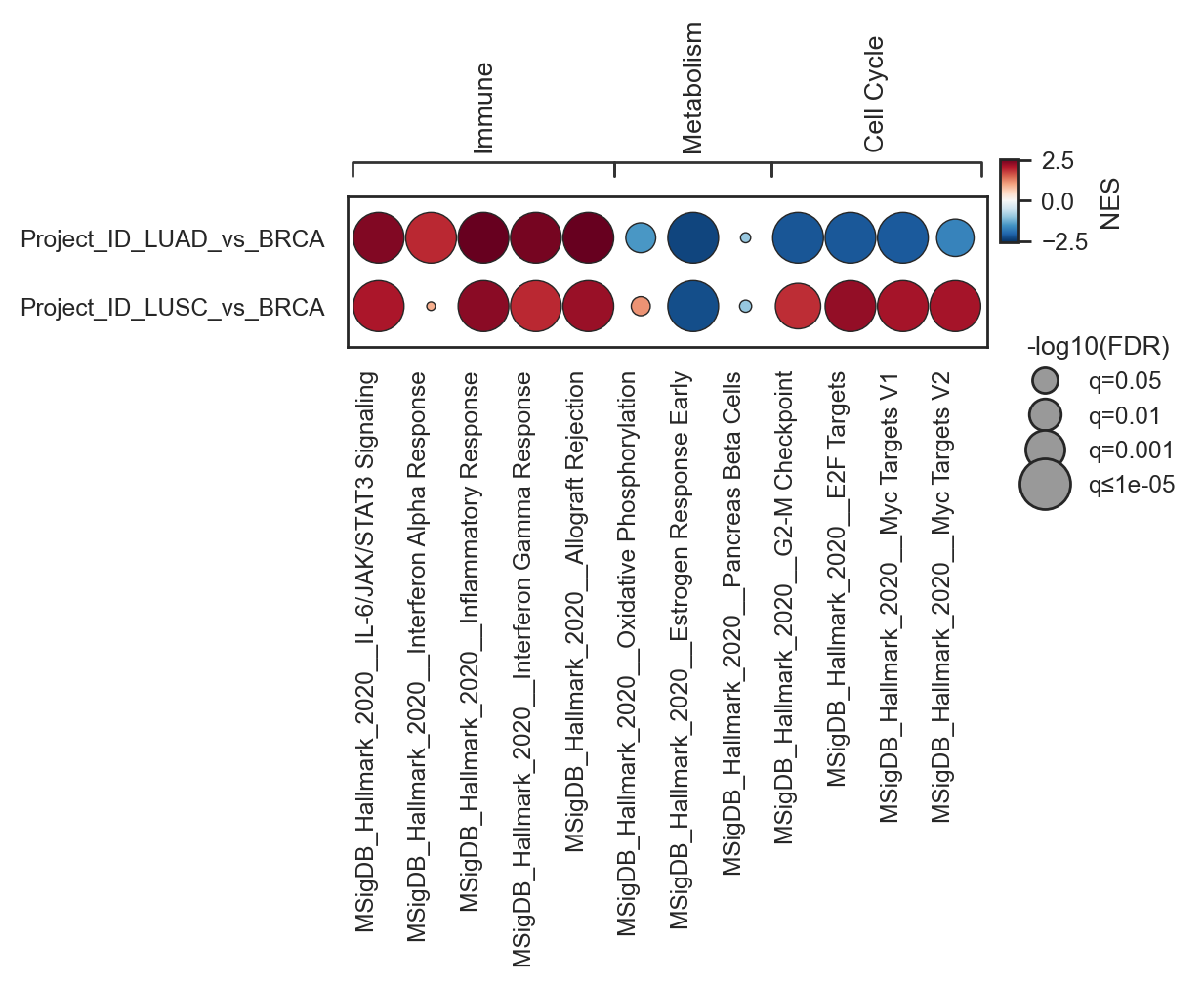
(<Figure size 1000x200 with 2 Axes>, <Axes: >)
10.6. Genesets, GO and GSEA Utilities#
10.6.1. Rerun GSEApy from previously saved rnk file#
(res not needed) only for plotting later:
rnk_path = "figs/gsea/RB1_mut_1.0_vs_0.0/RB1_mut_1.0_vs_0.0.rnk.tsv"
pre_res = gseapy.prerank(rnk=rnk_path, gene_sets="MSigDB_Hallmark_2020", outdir=None)
10.6.2. Original genesets from GSEA - MSigDB#
msig = Msigdb()
msig.list_category(dbver="2025.1.Hs")
['c1.all',
'c2.all',
'c2.cgp',
'c2.cp.biocarta',
'c2.cp.kegg_legacy',
'c2.cp.kegg_medicus',
'c2.cp.pid',
'c2.cp.reactome',
'c2.cp',
'c2.cp.wikipathways',
'c3.all',
'c3.mir.mir_legacy',
'c3.mir.mirdb',
'c3.mir',
'c3.tft.gtrd',
'c3.tft.tft_legacy',
'c3.tft',
'c4.3ca',
'c4.all',
'c4.cgn',
'c4.cm',
'c5.all',
'c5.go.bp',
'c5.go.cc',
'c5.go.mf',
'c5.go',
'c5.hpo',
'c6.all',
'c7.all',
'c7.immunesigdb',
'c7.vax',
'c8.all',
'h.all',
'msigdb']
h_all = msig.get_gmt(category='h.all', dbver="2025.1.Hs") # HALLMARKS
h_c2_all = msig.get_gmt(category='2.cp.reactome', dbver="2025.1.Hs")
print(h_all['HALLMARK_WNT_BETA_CATENIN_SIGNALING'])
10.6.3. Enrichr datasets#
The authoritative list is the Enrichr dataset Statistics endpoint. To discover exact names installed in your environment:
bk.tl.list_enrichr_libraries()[:50]
['ARCHS4_Cell-lines',
'ARCHS4_IDG_Coexp',
'ARCHS4_Kinases_Coexp',
'ARCHS4_TFs_Coexp',
'ARCHS4_Tissues',
'Achilles_fitness_decrease',
'Achilles_fitness_increase',
'Aging_Perturbations_from_GEO_down',
'Aging_Perturbations_from_GEO_up',
'Allen_Brain_Atlas_10x_scRNA_2021',
'Allen_Brain_Atlas_down',
'Allen_Brain_Atlas_up',
'Azimuth_2023',
'Azimuth_Cell_Types_2021',
'BioCarta_2013',
'BioCarta_2015',
'BioCarta_2016',
'BioPlanet_2019',
'BioPlex_2017',
'CCLE_Proteomics_2020',
'CM4AI_U2OS_Protein_Localization_Assemblies',
'COMPARTMENTS_Curated_2025',
'COMPARTMENTS_Experimental_2025',
'CORUM',
'COVID-19_Related_Gene_Sets',
'COVID-19_Related_Gene_Sets_2021',
'Cancer_Cell_Line_Encyclopedia',
'CellMarker_2024',
'CellMarker_Augmented_2021',
'ChEA_2013',
'ChEA_2015',
'ChEA_2016',
'ChEA_2022',
'Chromosome_Location',
'Chromosome_Location_hg19',
'ClinVar_2019',
'ClinVar_2025',
'DGIdb_Drug_Targets_2024',
'DSigDB',
'Data_Acquisition_Method_Most_Popular_Genes',
'DepMap_CRISPR_GeneDependency_CellLines_2023',
'DepMap_WG_CRISPR_Screens_Broad_CellLines_2019',
'DepMap_WG_CRISPR_Screens_Sanger_CellLines_2019',
'Descartes_Cell_Types_and_Tissue_2021',
'Diabetes_Perturbations_GEO_2022',
'DisGeNET',
'Disease_Perturbations_from_GEO_down',
'Disease_Perturbations_from_GEO_up',
'Disease_Signatures_from_GEO_down_2014',
'Disease_Signatures_from_GEO_up_2014']
11. Metaprograms and Tumor Heterogeneity#
11.1. Calculate and integrate metaprogram scores#
Load the published MPs (no refitting):
Gavish et al. Nature volume 618, pages598–606 (2023): https://www.nature.com/articles/s41586-023-06130-4
NP gene tables in: https://www.weizmann.ac.il/sites/3CA/search-genes
mp_dict = bk.tl.read_metaprograms_xlsx(
"../data/mp/meta_programs_2025-01-29.xlsx",
sheet_name="Malignant",
min_genes=10
)
len(mp_dict), list(mp_dict)[:5]
(67,
['MP1 Cell Cycle - G2/M',
'MP2 Cell Cycle - G1/S',
'MP3 Cell Cylce HMG-rich',
'MP4 Chromatin',
'MP5 Cell cycle single-nucleus'])
Score MPs per sample (bulk)
df_mp_scores, df_mp_info = bk.tl.score_metaprograms(
adata,
mp_dict,
layer="log1p_cpm",
zscore_genes=True,
min_genes_found=8,
prefix="MP_",
obsm_key="X_mp",
add_obs=True,
)
df_mp_info.head(10)
| mp | n_genes_listed | n_genes_found | genes_found | kept | reason | |
|---|---|---|---|---|---|---|
| 0 | MP1 Cell Cycle - G2/M | 50 | 50 | [HMGB2, UBE2C, NUSAP1, PTTG1, CKS2, KPNA2, SMC... | True | |
| 1 | MP2 Cell Cycle - G1/S | 50 | 50 | [PCNA, FEN1, MCM3, TYMS, GMNN, TK1, RRM1, RFC4... | True | |
| 2 | MP3 Cell Cylce HMG-rich | 50 | 50 | [STMN1, TUBA1B, H2AFZ, RANBP1, NME1, RAN, PTTG... | True | |
| 3 | MP6 Stress 1 | 50 | 50 | [EGR1, FOS, JUN, IER2, DUSP1, FOSB, ATF3, PPP1... | True | |
| 4 | MP10 Proteasomal degradation | 50 | 50 | [CCT5, CCT7, CCT8, MDH1, PRMT1, PSMC4, SSB, PS... | True | |
| 5 | MP12 Protein maturation | 50 | 50 | [HSPA5, LGALS3BP, PDIA3, GRN, PDIA6, TMEM59, A... | True | |
| 6 | MP15 EMT-I | 50 | 50 | [COL1A2, SPARC, COL1A1, FN1, COL3A1, COL6A2, I... | True | |
| 7 | MP16 EMT-II | 50 | 50 | [LAMC2, LAMB3, KRT17, LAMA3, LGALS1, MT2A, PME... | True | |
| 8 | MP17 EMT-III | 50 | 50 | [S100A6, ANXA2, LGALS1, S100A10, ANXA1, EMP3, ... | True | |
| 9 | MP22 Interferon/MHC-II (I) | 50 | 50 | [CD74, ISG15, HLA-DRB1, HLA-DRA, STAT1, IFI6, ... | True |
adata.obs.head(3)
| Patient_ID | Project_ID | gender | race | ajcc_pathologic_tumor_stage | clinical_stage | histological_type | histological_grade | initial_pathologic_dx_year | menopause_status | ... | MP_MP58_Metal_response | MP_MP59_PDAC_related_1 | MP_MP60_PDAC_related_2 | MP_MP61_PDAC_related_3 | MP_MP62_PDAC_related_4 | MP_MP63_PDAC_related_5 | MP_MP64_Adherens | MP_MP65_Cholesterol_Homeostasis | MP_MP66_Unassigned_1 | MP_MP67_Unassigned_2 | |
|---|---|---|---|---|---|---|---|---|---|---|---|---|---|---|---|---|---|---|---|---|---|
| Sample_ID | |||||||||||||||||||||
| TCGA-S9-A7J2-01 | TCGA-S9-A7J2 | LGG | MALE | WHITE | NaN | NaN | Oligodendroglioma | G3 | 2013.0 | NaN | ... | -0.467893 | -1.212706 | -0.665682 | -0.505248 | -0.580963 | -0.386989 | -0.376297 | 0.075637 | -0.135036 | 0.337450 |
| TCGA-G3-A3CH-11 | TCGA-G3-A3CH | LIHC | MALE | ASIAN | Stage IIIA | NaN | Hepatocellular Carcinoma | G2 | 2010.0 | NaN | ... | -0.150010 | -0.171668 | -0.462129 | 0.373682 | -0.114546 | -0.640391 | -0.802499 | 0.414227 | -0.338817 | -0.516038 |
| TCGA-EK-A2RE-01 | TCGA-EK-A2RE | CESC | FEMALE | WHITE | NaN | Stage IIA | Cervical Squamous Cell Carcinoma | G2 | 2010.0 | Pre (<6 months since LMP AND no prior bilatera... | ... | 0.131827 | 0.515806 | 0.583037 | -0.447925 | -0.729030 | 0.193594 | 0.968015 | 0.494608 | -0.336855 | -0.264538 |
3 rows × 1182 columns
QC / sanity checks
check how many genes found per MP
check score distributions
check correlation among MPs (some will correlate strongly)
# genes found distribution
df_mp_info[df_mp_info["kept"]][["mp","n_genes_found"]].describe()
| n_genes_found | |
|---|---|
| count | 67.000000 |
| mean | 48.776119 |
| std | 1.422981 |
| min | 43.000000 |
| 25% | 48.000000 |
| 50% | 49.000000 |
| 75% | 50.000000 |
| max | 50.000000 |
# MP score correlation
mp_corr = df_mp_scores.corr()
mp_corr.head(3)
| MP1 Cell Cycle - G2/M | MP2 Cell Cycle - G1/S | MP3 Cell Cylce HMG-rich | MP4 Chromatin | MP5 Cell cycle single-nucleus | MP6 Stress 1 | MP7 Hypoxia | MP8 Stress (in vitro) | MP9 Stress 2 | MP10 Proteasomal degradation | ... | MP58 Metal-response | MP59 PDAC-related 1 | MP60 PDAC-related 2 | MP61 PDAC-related 3 | MP62 PDAC-related 4 | MP63 PDAC-related 5 | MP64 Adherens | MP65 Cholesterol Homeostasis | MP66 Unassigned 1 | MP67 Unassigned 2 | |
|---|---|---|---|---|---|---|---|---|---|---|---|---|---|---|---|---|---|---|---|---|---|
| MP1 Cell Cycle - G2/M | 1.000000 | 0.963519 | 0.788681 | 0.142573 | 0.910663 | -0.036102 | 0.091020 | 0.283736 | 0.504685 | 0.586114 | ... | -0.119713 | 0.233277 | 0.139070 | 0.035847 | -0.068644 | 0.195026 | 0.273557 | 0.292962 | -0.016872 | -0.032426 |
| MP2 Cell Cycle - G1/S | 0.963519 | 1.000000 | 0.787357 | 0.165466 | 0.928671 | -0.062871 | 0.050651 | 0.271971 | 0.474063 | 0.574377 | ... | -0.165347 | 0.175966 | 0.082685 | -0.017815 | -0.121357 | 0.159132 | 0.257276 | 0.254432 | -0.017673 | 0.012287 |
| MP3 Cell Cylce HMG-rich | 0.788681 | 0.787357 | 1.000000 | -0.237498 | 0.597231 | -0.048011 | 0.094787 | 0.459926 | 0.518897 | 0.876565 | ... | -0.004582 | 0.166834 | 0.026054 | -0.008847 | -0.128772 | 0.001081 | 0.028813 | 0.297179 | -0.269764 | 0.074389 |
3 rows × 67 columns
Heterogeneity per tumor group + downstream association
df_het = bk.tl.metaprogram_heterogeneity(
adata,
groupby="Project_ID",
stat="sd",
)
df_het.head(3)
| group | mp | mean | heterogeneity_sd | n | |
|---|---|---|---|---|---|
| 0 | ACC | MP1 | -0.261250 | 0.698953 | 77 |
| 1 | ACC | MP2 | -0.350239 | 0.667997 | 77 |
| 2 | ACC | MP3 | -0.000855 | 0.429767 | 77 |
# Example: for each project, overall MP heterogeneity summary
df_project_summary = (
df_het.groupby("group")["heterogeneity_sd"]
.agg(["mean","median","max"])
.reset_index()
)
df_project_summary.head()
| group | mean | median | max | |
|---|---|---|---|---|
| 0 | ACC | 0.308101 | 0.285822 | 0.698953 |
| 1 | BLCA | 0.371148 | 0.353514 | 0.808845 |
| 2 | BRCA | 0.324083 | 0.285832 | 0.669480 |
| 3 | CESC | 0.335568 | 0.313953 | 0.692099 |
| 4 | CHOL | 0.356370 | 0.320541 | 1.036171 |
Then you can correlate:
MP scores (sample-level) with therapy response / NR@6m
MP heterogeneity (group-level) with prognosis metrics or resistance rates
Plots
# 1) after you ran bk.tl.score_metaprograms(...) storing adata.obsm["X_mp"]
df_corr = bk.pl.metaprogram_corr(
adata,
obsm_key="X_mp",
method="pearson",
cluster=True,
figsize=(12, 10),
)
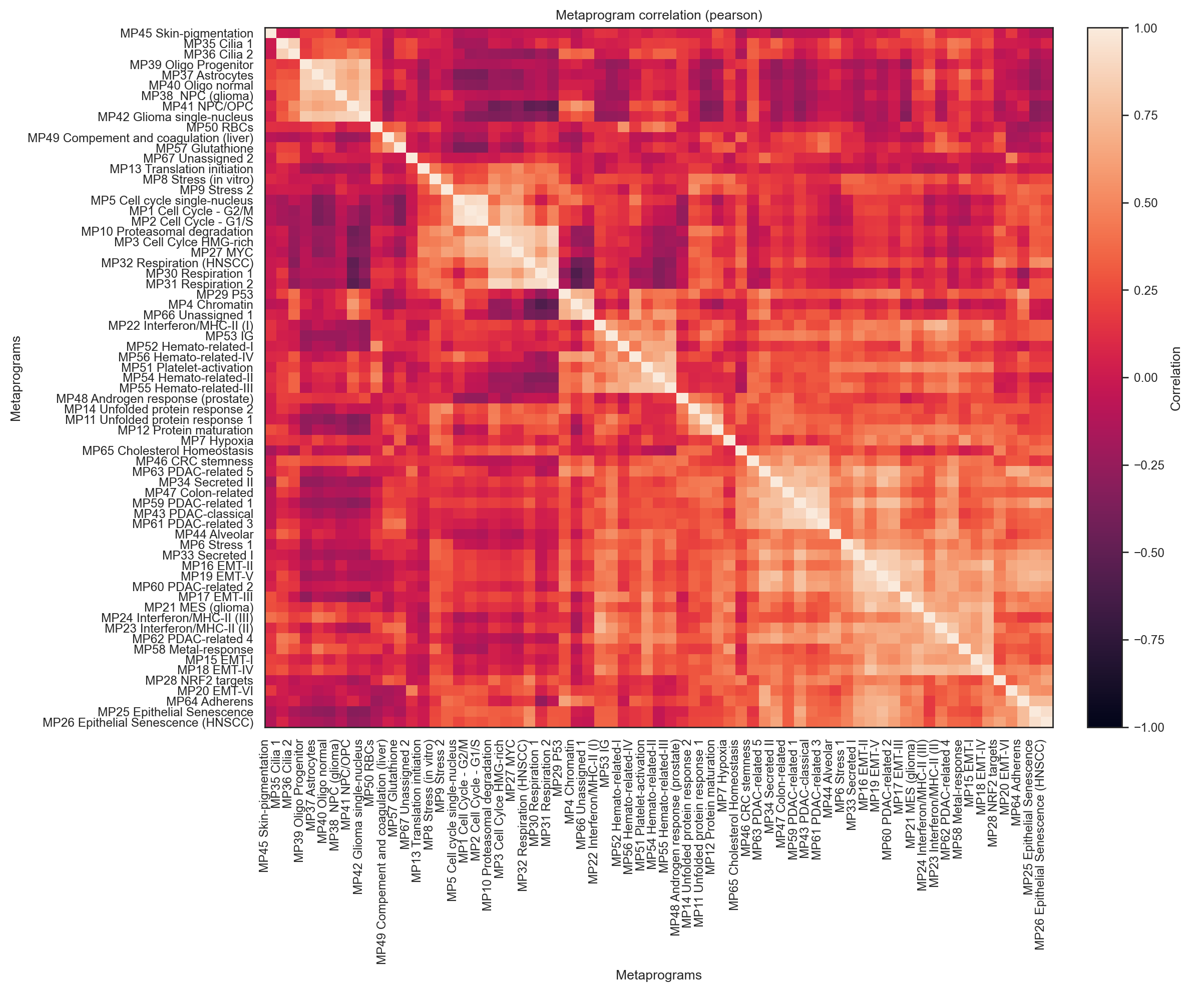
# 2) heatmap aggregated by tumor type
df_heat, df_group = bk.pl.metaprogram_heatmap(
adata,
obsm_key="X_mp",
groupby="Project_ID",
agg="mean",
scale="zscore_cols",
order_mps="cluster",
order_groups="cluster", # # "size", "alpha", None, "cluster"
row_dendrogram=True,
col_dendrogram=True,
dendrogram_ratio=(0.1, 0.05), # (row_dendro_width, col_dendro_height) in figure fraction-ish
row_dendro_width=0.1,
col_dendro_height=0.18,
dendro_gap=0.07,
ytick_pad=1,
rotate_xticks=90,
figsize=(11, 5),
)
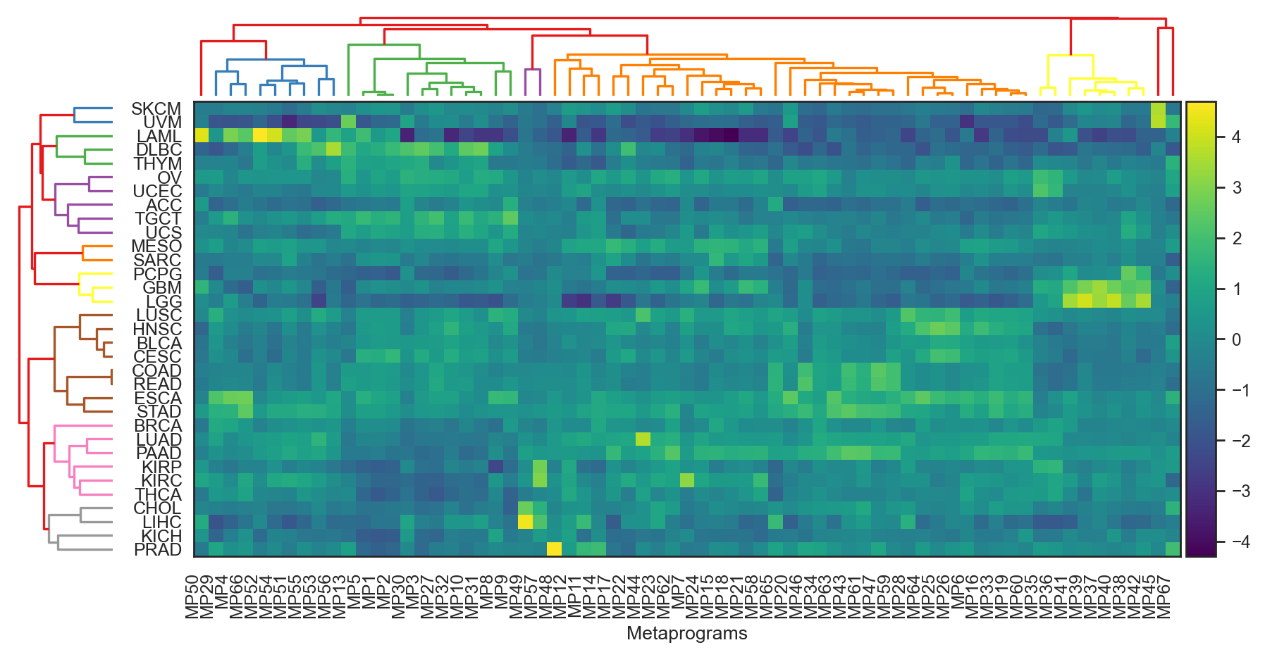
df_heat, df_group = bk.pl.metaprogram_heatmap(
adata,
groupby="Project_ID",
order_groups="cluster",
order_mps="cluster",
row_dendrogram=True,
col_dendrogram=True,
dendrogram_ratio=(0.1, 0.05), # (row_dendro_width, col_dendro_height) in figure fraction-ish
row_dendro_width=0.1,
col_dendro_height=0.18,
dendro_gap=0.07,
ytick_pad=1,
)
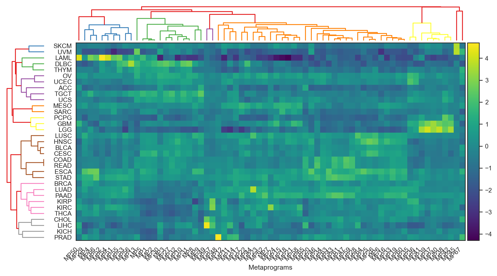
df_heat, df_group = bk.pl.metaprogram_heatmap(
adata,
groupby="Project_ID",
order_groups="alpha", #"cluster"
order_mps="cluster",
row_dendrogram=False,
col_dendrogram=False,
rotate_xticks=90,
figsize=(12, 7),
)
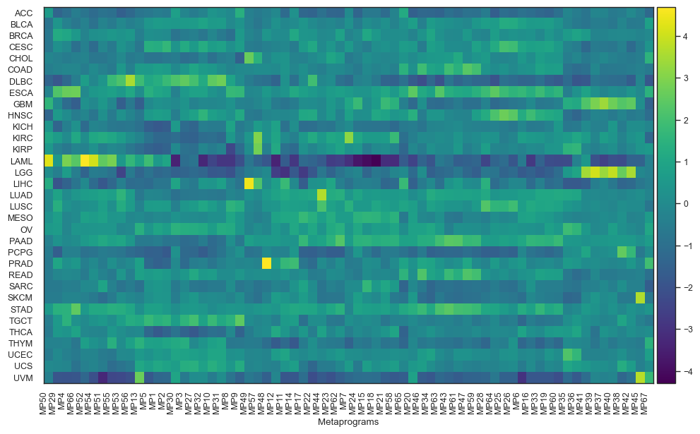
11.2. Functional tumor heterogeneity and dispersion in metaprograms#
# 1) compute per-sample metaprogram heterogeneity + dispersion
bk.tl.metaprogram_sample_metrics(
adata,
groupby="Project_ID",
out_prefix="mp",
heterogeneity="entropy",
dispersion="mad",
zscore_within_group=True,
)
# 2) compute per-group metaprogram dispersion table
bk.tl.metaprogram_dispersion_by_group(adata, groupby="Project_ID", method="mad")
| group | metaprogram | dispersion | n | |
|---|---|---|---|---|
| 0 | ACC | MP1 | 0.520609 | 77 |
| 1 | ACC | MP2 | 0.444303 | 77 |
| 2 | ACC | MP3 | 0.283294 | 77 |
| 3 | ACC | MP4 | 0.227157 | 77 |
| 4 | ACC | MP5 | 0.398499 | 77 |
| ... | ... | ... | ... | ... |
| 2206 | UVM | MP63 | 0.085296 | 79 |
| 2207 | UVM | MP64 | 0.109303 | 79 |
| 2208 | UVM | MP65 | 0.088886 | 79 |
| 2209 | UVM | MP66 | 0.293019 | 79 |
| 2210 | UVM | MP67 | 0.157194 | 79 |
2211 rows × 4 columns
# 3) optional: link metaprograms to NE signature score
bk.tl.metaprogram_ne_enrichment(adata, ne_signature_key="Neuroendocrine_score")
| metaprogram | rho | pval | n | qval | |
|---|---|---|---|---|---|
| 0 | MP39 | 0.371733 | 0.000000e+00 | 10534 | 0.000000e+00 |
| 1 | MP55 | -0.366421 | 0.000000e+00 | 10534 | 0.000000e+00 |
| 2 | MP66 | -0.379799 | 0.000000e+00 | 10534 | 0.000000e+00 |
| 3 | MP54 | -0.304640 | 4.542518e-225 | 10534 | 7.608718e-224 |
| 4 | MP62 | -0.292750 | 3.240619e-207 | 10534 | 4.342430e-206 |
| ... | ... | ... | ... | ... | ... |
| 62 | MP5 | -0.017152 | 7.835204e-02 | 10534 | 8.332677e-02 |
| 63 | MP8 | -0.013691 | 1.600044e-01 | 10534 | 1.675047e-01 |
| 64 | MP11 | -0.013510 | 1.655960e-01 | 10534 | 1.706912e-01 |
| 65 | MP41 | 0.005333 | 5.841821e-01 | 10534 | 5.930334e-01 |
| 66 | MP14 | -0.004431 | 6.493322e-01 | 10534 | 6.493322e-01 |
67 rows × 5 columns
# 4) optional: compute top-k dominance per sample
bk.tl.metaprogram_topk_contribution(adata, k=3)
| sample | rank | metaprogram | weight | score | |
|---|---|---|---|---|---|
| 0 | TCGA-S9-A7J2-01 | 1 | MP39 | 0.099434 | 1.801954 |
| 1 | TCGA-S9-A7J2-01 | 2 | MP42 | 0.083157 | 1.623190 |
| 2 | TCGA-S9-A7J2-01 | 3 | MP37 | 0.075905 | 1.531936 |
| 3 | TCGA-G3-A3CH-11 | 1 | MP49 | 0.347304 | 3.383460 |
| 4 | TCGA-G3-A3CH-11 | 2 | MP57 | 0.052549 | 1.495013 |
| ... | ... | ... | ... | ... | ... |
| 31597 | TCGA-DD-A115-01 | 2 | MP57 | 0.037155 | 1.129155 |
| 31598 | TCGA-DD-A115-01 | 3 | MP65 | 0.022571 | 0.630744 |
| 31599 | TCGA-FV-A3I0-11 | 1 | MP49 | 0.372073 | 3.470628 |
| 31600 | TCGA-FV-A3I0-11 | 2 | MP57 | 0.046873 | 1.398979 |
| 31601 | TCGA-FV-A3I0-11 | 3 | MP6 | 0.028600 | 0.904930 |
31602 rows × 5 columns
obsm[“X_mp”] likely has no column names stored. Since you also have metaprograms as .obs columns (MP_MP1_… etc.), you can sync names
#mp_cols = [c for c in adata.obs.columns if c.startswith("MP_")]
#adata.uns["metaprogram_names"] = mp_cols
Dispersion plots#
Heatmap: metaprogram dispersion by tumor type#
Identify which tumors show highest program variability; highlight NE-related or other MPs later.
bk.pl.metaprogram_dispersion_heatmap(adata, figsize=(4,8),
save=DESKTOP + "metaprogram_dispersion.png")
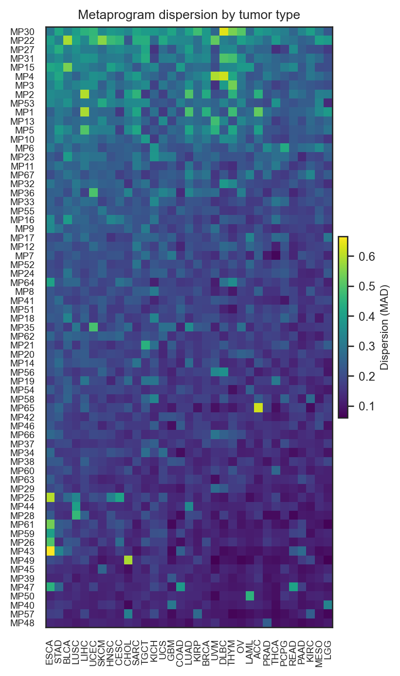
<Axes: title={'center': 'Metaprogram dispersion by tumor type'}>
Summary: heterogeneity + dispersion by tumor type (two boxplots)#
Show cohort-level differences in “program mixture” (entropy) and dispersion.
bk.pl.metaprogram_metrics_summary(adata,
save=DESKTOP + "metaprogram_metrics.png")
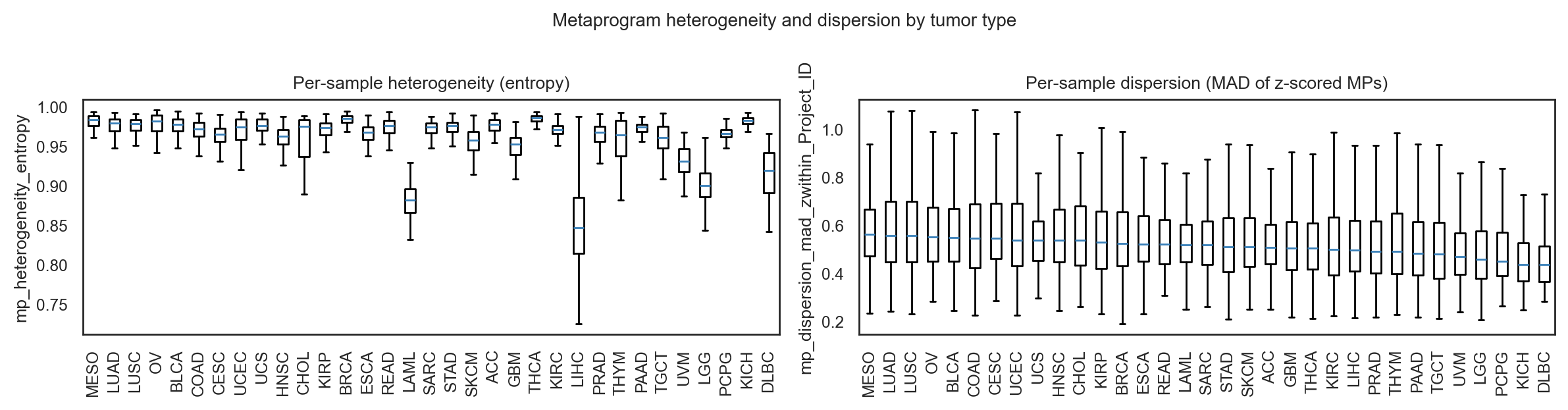
array([<Axes: title={'center': 'Per-sample heterogeneity (entropy)'}, ylabel='mp_heterogeneity_entropy'>,
<Axes: title={'center': 'Per-sample dispersion (MAD of z-scored MPs)'}, ylabel='mp_dispersion_mad_zwithin_Project_ID'>],
dtype=object)
Scatter: NE score vs metaprogram heterogeneity (or dispersion)#
“NE ↔ heterogeneity” centerpiece.
NE vs heterogeneity entropy#
bk.pl.metaprogram_ne_scatter(adata, ne_key="Proliferation_score", x_key="mp_heterogeneity_entropy", figsize=(3.5,3.5),
save= DESKTOP + "metaprogram_entropy_scatter.png")
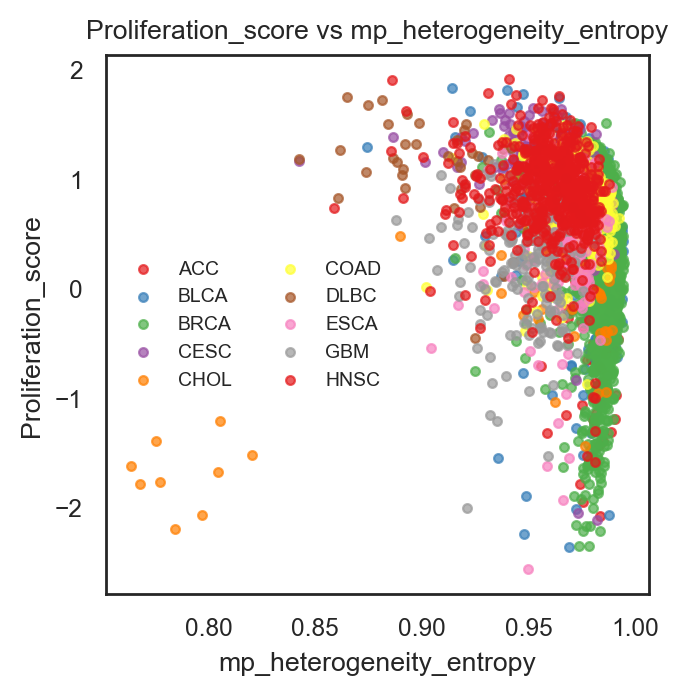
<Axes: title={'center': 'Proliferation_score vs mp_heterogeneity_entropy'}, xlabel='mp_heterogeneity_entropy', ylabel='Proliferation_score'>
NE vs dispersion#
ax = bk.pl.metaprogram_ne_scatter(
adata,
ne_key="Proliferation_score",
x_key="mp_dispersion_mad_zwithin_Project_ID",
groupby="Project_ID",
max_groups=10,
title="Neuroendocrine program vs metaprogram dispersion",
show=True,
figsize=(3,3),
save=DESKTOP + "Fig_NE_vs_MP_dispersion.png",
)
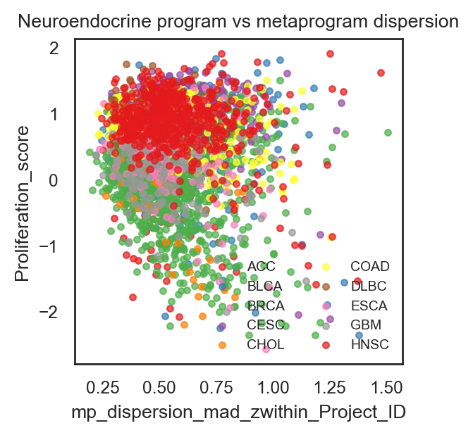
Dominance: top metaprogram weight distribution by tumor type#
Show whether tumors are dominated by one MP (low heterogeneity) vs distributed (high heterogeneity).
This uses adata.uns[“mp_topk”]. It plots the distribution of the rank-1 metaprogram weight per tumor type.
bk.tl.metaprogram_topk_contribution(adata)
| sample | rank | metaprogram | weight | score | |
|---|---|---|---|---|---|
| 0 | TCGA-S9-A7J2-01 | 1 | MP39 | 0.099434 | 1.801954 |
| 1 | TCGA-S9-A7J2-01 | 2 | MP42 | 0.083157 | 1.623190 |
| 2 | TCGA-S9-A7J2-01 | 3 | MP37 | 0.075905 | 1.531936 |
| 3 | TCGA-G3-A3CH-11 | 1 | MP49 | 0.347304 | 3.383460 |
| 4 | TCGA-G3-A3CH-11 | 2 | MP57 | 0.052549 | 1.495013 |
| ... | ... | ... | ... | ... | ... |
| 31597 | TCGA-DD-A115-01 | 2 | MP57 | 0.037155 | 1.129155 |
| 31598 | TCGA-DD-A115-01 | 3 | MP65 | 0.022571 | 0.630744 |
| 31599 | TCGA-FV-A3I0-11 | 1 | MP49 | 0.372073 | 3.470628 |
| 31600 | TCGA-FV-A3I0-11 | 2 | MP57 | 0.046873 | 1.398979 |
| 31601 | TCGA-FV-A3I0-11 | 3 | MP6 | 0.028600 | 0.904930 |
31602 rows × 5 columns
bk.pl.metaprogram_dominance_ridgeplot_like(
adata,
topk_key="mp_topk",
groupby="Project_ID",
weight_key= "weight",
rank=1,
#max_groups=12,
ylim=(0, 0.5),
#y_text=1, # None
fontsize=10,
figsize=(5, 3),
save=DESKTOP+"Fig_MP_rank1_dominance.png",
)
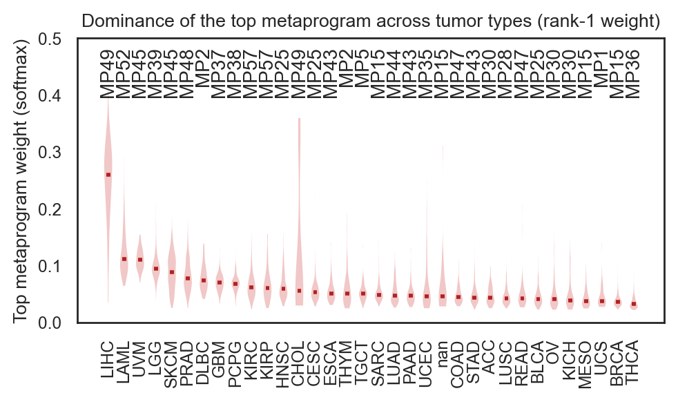
<Axes: title={'center': 'Dominance of the top metaprogram across tumor types (rank-1 weight)'}, ylabel='Top metaprogram weight (softmax)'>
bk.pl.metaprogram_rank1_composition_stackedbar(
adata,
topk_key="mp_topk",
groupby="Project_ID",
rank=1,
top_groups=12,
top_mps=12,
figsize=(6, 4),
legend=True,
legend_bbox_to_anchor=(2.15, 1.0),
legend_loc="upper right",
rotation=90,
title="Rank-1 metaprogram composition across tumor types",
ylabel="Fraction of samples where MP is rank-1",
show=True,
save=DESKTOP + "mp_stackedbar.png",
out_key="mp_rank1_composition",
)
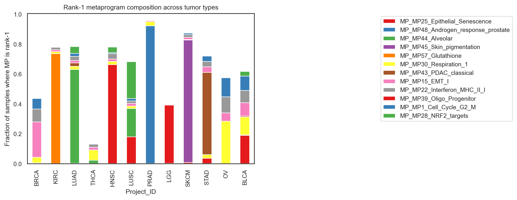
<Axes: title={'center': 'Rank-1 metaprogram composition across tumor types'}, xlabel='Project_ID', ylabel='Fraction of samples where MP is rank-1'>
limiting to the top ~10–15 MPs globally keeps the figure readable. You can add a “Other” category if you want.
11.3. Survival Analysis#
11.3.1. Cox univariate#
heterogeneity entropy, continuous values
adata.obs["Neuroendocrine_score"] = pd.to_numeric(adata.obs["Neuroendocrine_score"], errors="coerce")
res, models = bk.tl.cox_univariate(
adata,
time_key="OS.time",
event_key="OS",
x_keys=[
"mp_heterogeneity_entropy",
"mp_dispersion_mad_zwithin_Project_ID",
"Neuroendocrine_score",
"Proliferation_score",
],
x_mode="continuous",
strata="Project_ID",
out_key="cox_compare_candidates",
)
bk.pl.cox_forest_from_uns():
If uns is provided, adata can be None. If uns is None, adata must be provided and contain uns_key.
bk.pl.cox_forest_from_uns(
adata,
uns_key="cox_compare_candidates",
rename={
"mp_heterogeneity_entropy": "Metaprogram heterogeneity (entropy)",
"mp_dispersion_mad_zwithin_Project_ID": "Metaprogram dispersion (MAD, within tumor)",
"Neuroendocrine_score": "Neuroendocrine score",
"Proliferation_score": "Proliferation score",
},
sort_by="p",
xscale="log",
figsize=(5,1.5),
save=DESKTOP+"Fig_CoxForest_compare_predictors.png",
)
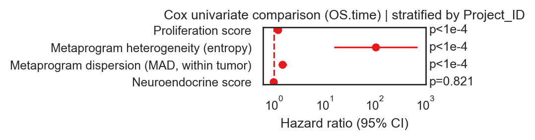
<Axes: title={'center': 'Cox univariate comparison (OS.time) | stratified by Project_ID'}, xlabel='Hazard ratio (95% CI)'>
Run cox per group (in Project_ID)#
cox_by_project = bk.pl.run_cox_per_group(
adata,
group_col="Project_ID",
min_n=30,
time_key="OS.time",
event_key="OS",
x_keys=[
"mp_heterogeneity_entropy",
"mp_dispersion_mad_zwithin_Project_ID",
"Neuroendocrine_score",
"Proliferation_score",
],
strata=None, # or e.g. strata="sex" if present within each tumor type
)
[OK] ACC: n=77 stored 'cox_ACC'
[OK] BLCA: n=426 stored 'cox_BLCA'
[OK] BRCA: n=1211 stored 'cox_BRCA'
[OK] CESC: n=309 stored 'cox_CESC'
[OK] CHOL: n=45 stored 'cox_CHOL'
[OK] COAD: n=329 stored 'cox_COAD'
[OK] DLBC: n=47 stored 'cox_DLBC'
[OK] ESCA: n=195 stored 'cox_ESCA'
[OK] GBM: n=165 stored 'cox_GBM'
[OK] HNSC: n=564 stored 'cox_HNSC'
[OK] KICH: n=91 stored 'cox_KICH'
[OK] KIRC: n=603 stored 'cox_KIRC'
[OK] KIRP: n=321 stored 'cox_KIRP'
[OK] LAML: n=173 stored 'cox_LAML'
[OK] LGG: n=522 stored 'cox_LGG'
[OK] LIHC: n=421 stored 'cox_LIHC'
[OK] LUAD: n=574 stored 'cox_LUAD'
[OK] LUSC: n=548 stored 'cox_LUSC'
[OK] MESO: n=87 stored 'cox_MESO'
[OK] OV: n=426 stored 'cox_OV'
[OK] PAAD: n=183 stored 'cox_PAAD'
[OK] PCPG: n=185 stored 'cox_PCPG'
[OK] PRAD: n=548 stored 'cox_PRAD'
[OK] READ: n=102 stored 'cox_READ'
[OK] SARC: n=264 stored 'cox_SARC'
[OK] SKCM: n=470 stored 'cox_SKCM'
[OK] STAD: n=450 stored 'cox_STAD'
[OK] TGCT: n=137 stored 'cox_TGCT'
[OK] THCA: n=571 stored 'cox_THCA'
[OK] THYM: n=121 stored 'cox_THYM'
[OK] UCEC: n=194 stored 'cox_UCEC'
[OK] UCS: n=57 stored 'cox_UCS'
[OK] UVM: n=79 stored 'cox_UVM'
for pid, res in cox_by_project.items():
bk.pl.cox_forest_from_uns(
adata=None,
uns=res, # now supported
title=f"{pid} – Cox univariate (OS)",
sort_by="name",
xscale="log",
figsize=(5, 1.5), # or None for auto-height
show=True,
save=DESKTOP + f"Fig_CoxForest_{pid}.png",
)
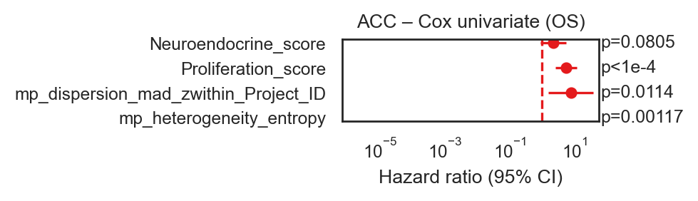
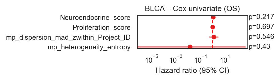
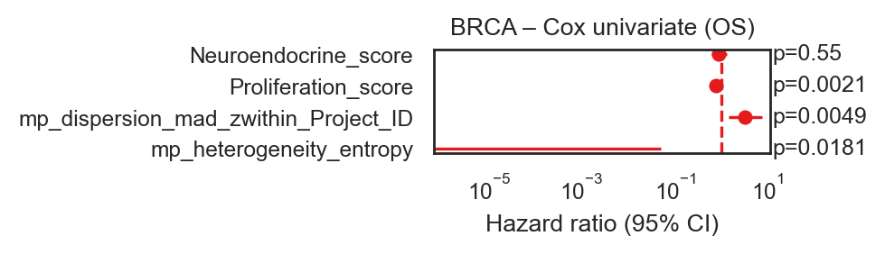
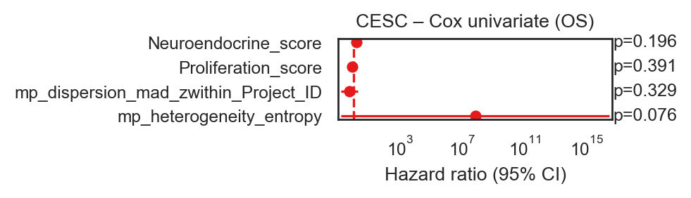
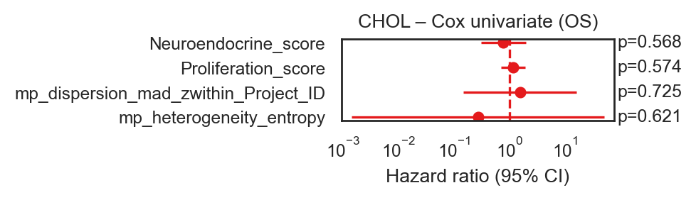
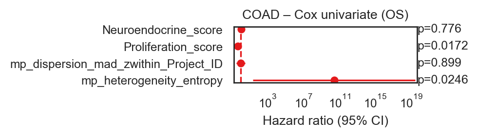
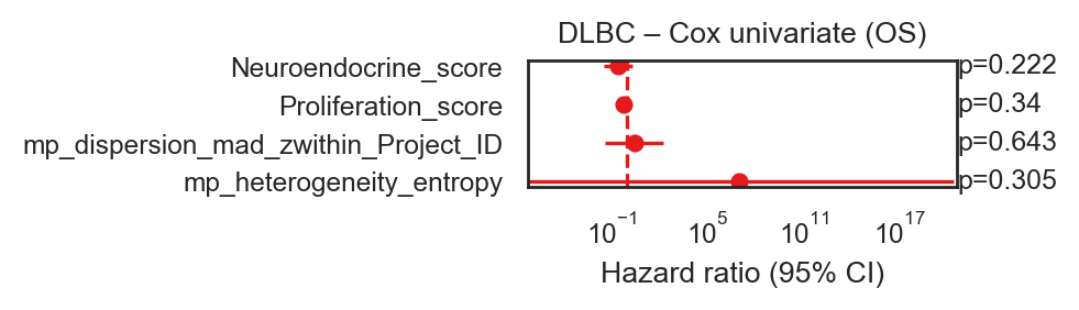
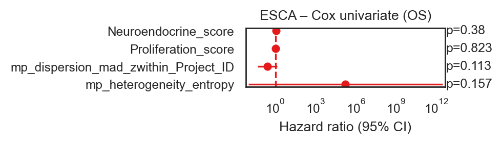
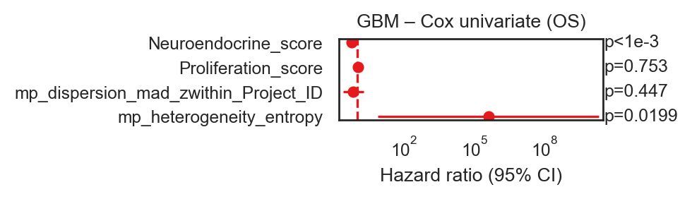
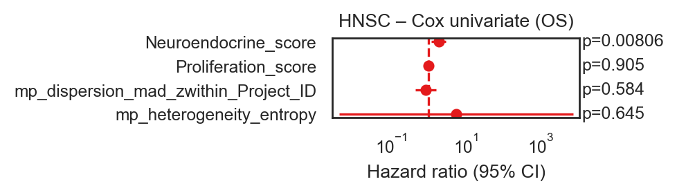
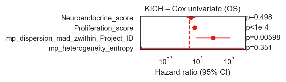
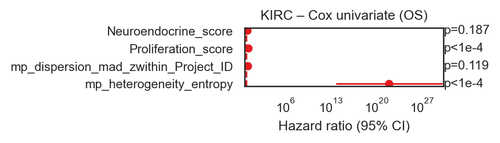
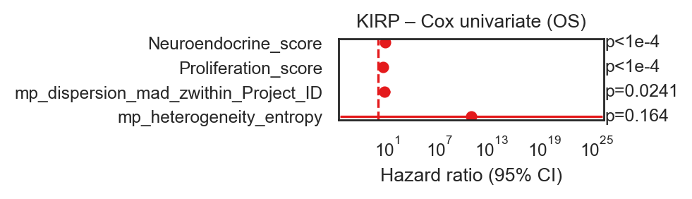
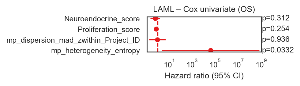
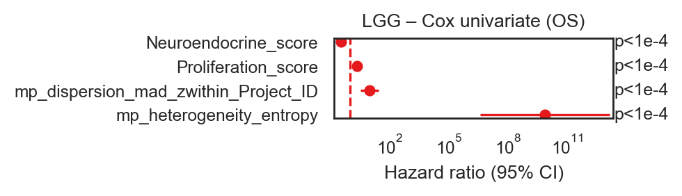
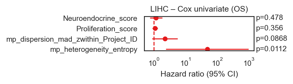
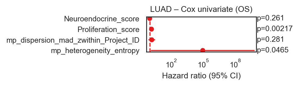
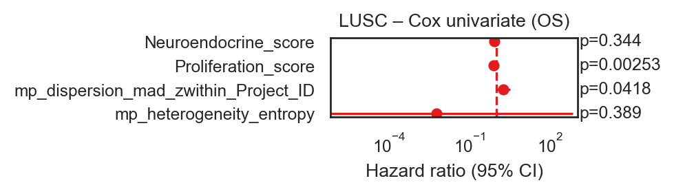
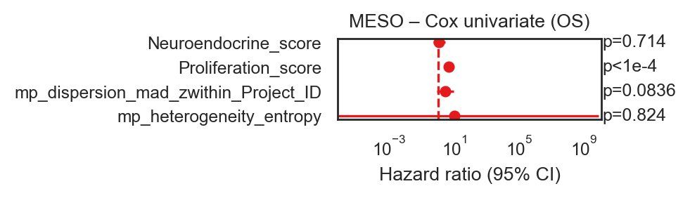
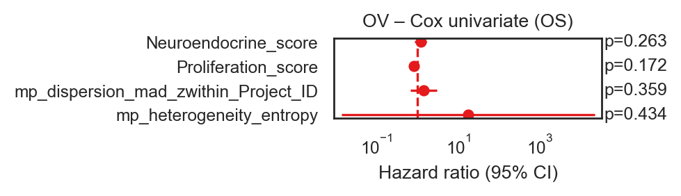
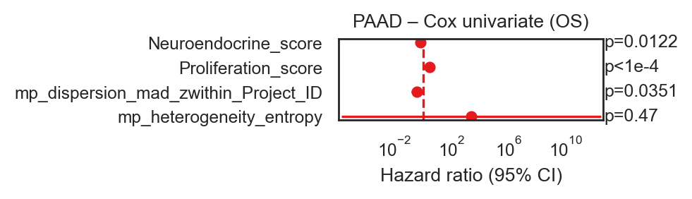
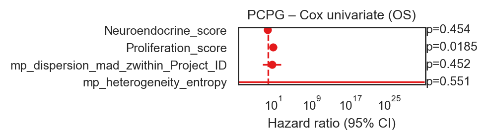
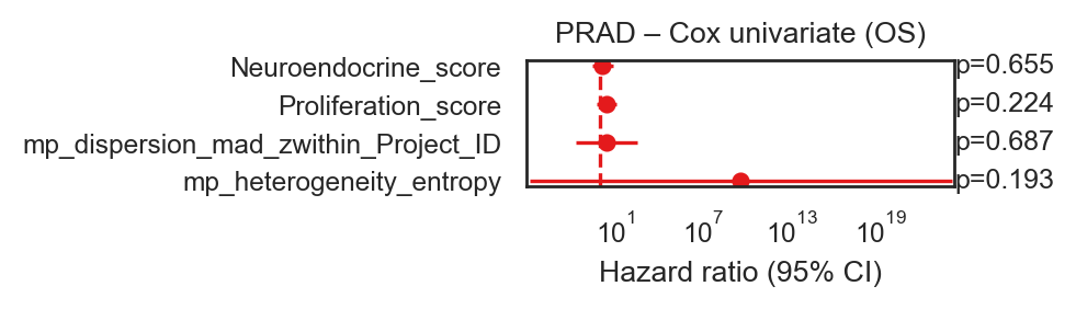
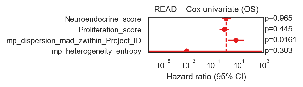
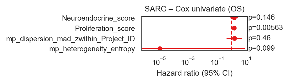
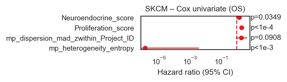
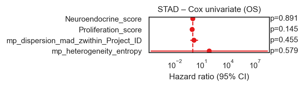
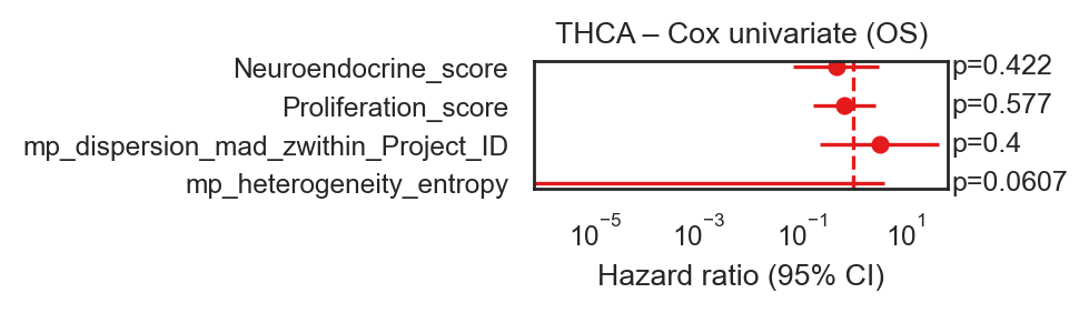
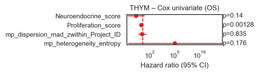
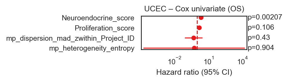
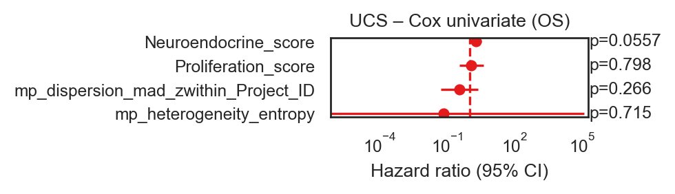
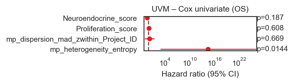
cox_by_project
def summarize_one_x_across_groups(cox_by_project: dict, x_key: str) -> dict:
rows = []
for pid, payload in cox_by_project.items():
summ = payload.get("summary", None)
if summ is None:
continue
if not isinstance(summ, pd.DataFrame):
summ = pd.DataFrame(summ)
# --- handle the “tidy multi-x” format ---
if "x_key" in summ.columns:
sub = summ[summ["x_key"].astype(str) == str(x_key)].copy()
if sub.shape[0] == 0:
continue
r = sub.iloc[0]
# --- handle “lifelines-like” single-model summary (indexed by covariate) ---
else:
if summ.index.name is None and "covariate" in summ.columns:
summ = summ.set_index("covariate")
if str(x_key) not in summ.index.astype(str):
continue
r = summ.loc[str(x_key)]
rows.append(
dict(
x_key=str(pid), # project name becomes x_key
term=str(x_key), # keep original covariate name
HR=float(r["HR"]),
HR_lower_95=float(r["HR_lower_95"]),
HR_upper_95=float(r["HR_upper_95"]),
p=float(r.get("p", np.nan)),
n_used=float(r.get("n_used", np.nan)),
events=float(r.get("events", np.nan)),
)
)
df = pd.DataFrame(rows)
return {
"summary": df,
"params": {"time_key": "OS.time", "strata": None, "note": f"{x_key} across groups"},
}
uns_one = summarize_one_x_across_groups(cox_by_project, "mp_heterogeneity_entropy")
ax = bk.pl.cox_forest_from_uns(
adata=None, # if your updated function allows
uns=uns_one, # <-- pass directly
title="Cox HR for mp_heterogeneity_entropy across tumor types",
sort_by="HR", # or "p" or "name"
xscale="log", # recommended for HR
figsize=(4, 0.1 * len(uns_one["summary"]) + 0.9),
show=True,
save="Fig_CoxForest_mp_heterogeneity_byProject.svg",
)
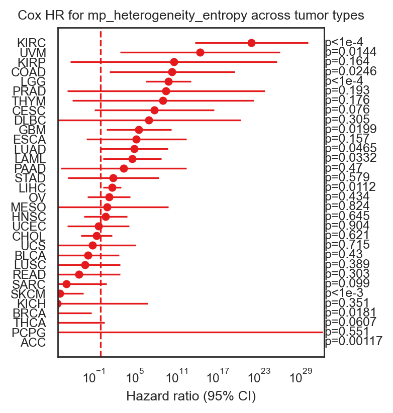
keep only projects with enough events or significant p-values
df = uns_one["summary"].copy()
df = df[df["events"].fillna(0) >= 20] # example
uns_one["summary"] = df
ax = bk.pl.cox_forest_from_uns(
adata=None, # if your updated function allows
uns=uns_one, # <-- pass directly
title="Cox HR for mp_heterogeneity_entropy across tumor types",
sort_by="HR", # or "p" or "name"
xscale="log", # recommended for HR
figsize=(4, 0.1 * len(uns_one["summary"]) + 0.8),
show=True,
save="Fig_CoxForest_mp_heterogeneity_byProject.svg",
)
ax.set_xlim(, 3.0)
plt.show()
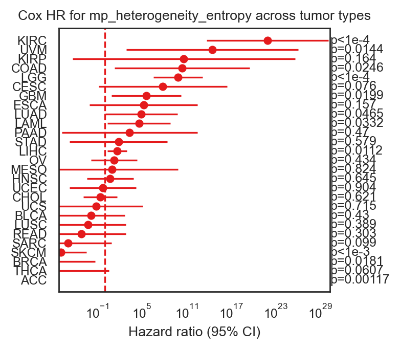
Binary extremes (if you prefer)
bk.tl.cox_univariate(
adata,
x_keys=["mp_heterogeneity_entropy", "Neuroendocrine_score"],
x_mode="binary",
q=(0.25, 0.75),
binning="global",
strata="Project_ID",
out_key="cox_compare_binary",
)
( x_key term coef HR HR_lower_95 \
0 mp_heterogeneity_entropy x_bin 0.056249 1.057861 0.899238
1 Neuroendocrine_score x_bin 0.151970 1.164126 0.993254
HR_upper_95 p n_used events
0 1.244466 0.497379 5172 1554
1 1.364393 0.060602 5172 1579 ,
{'mp_heterogeneity_entropy': <lifelines.CoxPHFitter: fitted with 5172 total observations, 3618 right-censored observations>,
'Neuroendocrine_score': <lifelines.CoxPHFitter: fitted with 5172 total observations, 3593 right-censored observations>})
bk.pl.cox_forest_from_uns(
adata,
uns_key="cox_compare_binary",
sort_by="HR",
save="Fig_CoxForest_compare_binary.svg",
)

<Axes: title={'center': 'Cox univariate comparison (OS.time) | stratified by Project_ID'}, xlabel='Hazard ratio (95% CI)'>
11.3.2. Kaplan-Meier curves#
Uses module lifetimes: - https://pypi.org/project/Lifetimes/
2×2 interaction” Kaplan–Meier: NE-high/low × heterogeneity-high/low
This is a killer figure for the story (and it’s simple).
If you want, tell me which survival endpoint you prefer (OS, DSS, PFI) and I’ll give you the exact code that:
• bins NE and heterogeneity into high/low (e.g., quartiles),
• builds 4 groups,
• plots KM + Cox interaction
adata_coad = adata[adata.obs.Project_ID == "COAD"]
cph, df_used = bk.tl.cox_interaction(
adata,
time_key="OS.time",
event_key="OS",
x_key="Proliferation_score",
z_key="mp_heterogeneity_entropy",
strata="Project_ID", # stratified baseline hazards by tumor type
binning="global", # or "global"within_group
q=(0.25, 0.75),
keep="extremes",
covariates=None, # e.g. ["gender", "Age at Diagnosis in Years"] after cleaning
out_key="cox_NE_x_mphet_OS",
)
# Print HRs
print(adata.uns["cox_NE_x_mphet_OS"]["summary"])
# Forest plot
fig, ax = plt.subplots(figsize=(2,1))
ax = cph.plot(hazard_ratios=True)
ax.figure.savefig("Fig_Cox_NE_x_Heterogeneity.svg", bbox_inches="tight")
plt.show()
coef HR HR_lower_95 HR_upper_95 p
covariate
x_bin 0.200441 1.221942 0.840185 1.777159 0.294266
z_bin 0.095053 1.099718 0.649396 1.862312 0.723586
x_z -0.134456 0.874191 0.494289 1.546080 0.643947
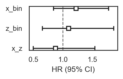
fig, ax = plt.subplots(figsize=(3,2), dpi=200)
ax = cph.plot(hazard_ratios=True)
ax.set_title("Stratified Cox model: NE × Metaprogram heterogeneity")
# ax.figure.savefig("Fig_Cox_NE_x_Heterogeneity.svg", bbox_inches="tight")
Text(0.5, 1.0, 'Stratified Cox model: NE × Metaprogram heterogeneity')
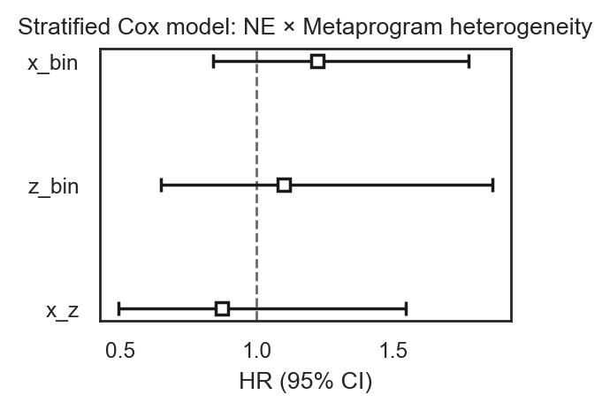
KM Univariate#
Produces:
• KM curves (low vs high)
• Log-rank p-value on plot
• adata.uns["km_1d"]["logrank_p"] stored for Results text
bk.pl.km_univariate(
adata,
x_key="Proliferation_score",
time_key="OS.time",
event_key="OS",
logrank=True,
figsize=(3, 3),
save="Fig_KM_Heterogeneity_OS.svg",
)
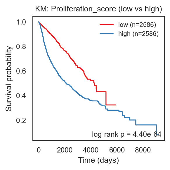
<Axes: title={'center': 'KM: Proliferation_score (low vs high)'}, xlabel='Time (days)', ylabel='Survival probability'>
bk.pl.km_univariate(
adata,
x_key="RB1_mut",
x_source="obs",
binary_mode="auto", # or "force"
binary_labels=("WT", "Mut"),
palette={"0":"tab:blue", "1":"tab:red"},
min_n=20,
figsize=(3, 3),
logrank=True,
)
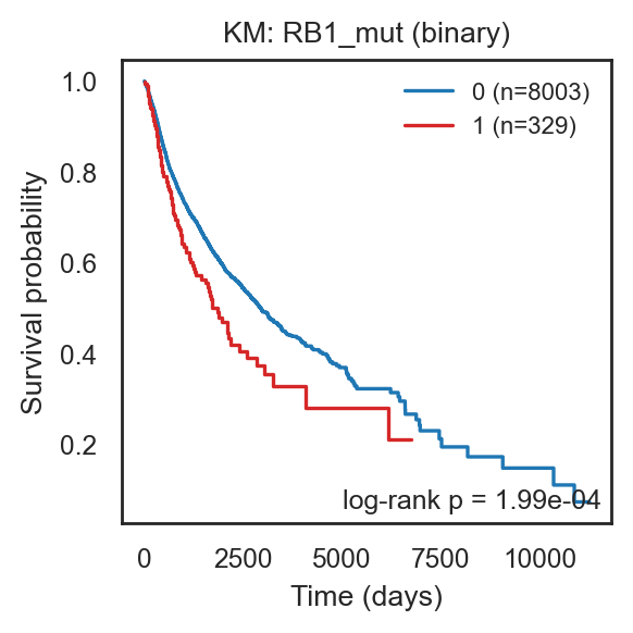
<Axes: title={'center': 'KM: RB1_mut (binary)'}, xlabel='Time (days)', ylabel='Survival probability'>
bk.pl.km_univariate(
adata,
x_key="RB1_mut",
time_key="OS.time",
event_key="OS",
logrank=True,
figsize=(3, 3),
save="Fig_KM_Heterogeneity_OS.svg",
)
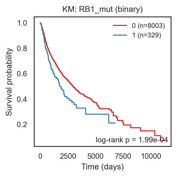
<Axes: title={'center': 'KM: RB1_mut (binary)'}, xlabel='Time (days)', ylabel='Survival probability'>
bk.pl.km_univariate(
adata,
x_key="mp_heterogeneity_entropy",
palette=("tab:blue", "tab:orange"), # low, high
logrank=True,
)
---------------------------------------------------------------------------
KeyError Traceback (most recent call last)
Cell In[13], line 1
----> 1 bk.pl.km_univariate(
2 adata,
3 x_key="mp_heterogeneity_entropy",
4 palette=("tab:blue", "tab:orange"), # low, high
5 logrank=True,
6 )
File ~/Library/CloudStorage/OneDrive-VHIO/BioInformatics/BioProjects/MM01_BULLKpy/bullkpy-skeleton/src/bullkpy/pl/cox.py:1722, in km_univariate(adata, x_key, x_source, layer, time_key, event_key, group_col, groupby_for_binning, binning, q, keep, labels, min_n, figsize, ylim, title, logrank, annotate_p, show, save, out_key, force_rebin, cleanup_tmp_cols, binary_mode, binary_labels, palette)
1720 # resolve x
1721 tmp_cols = []
-> 1722 x_src = _resolve_source(x_key, x_source)
1723 x_obs_key = x_key
1724 if x_src == "gene":
File ~/Library/CloudStorage/OneDrive-VHIO/BioInformatics/BioProjects/MM01_BULLKpy/bullkpy-skeleton/src/bullkpy/pl/cox.py:1693, in km_univariate.<locals>._resolve_source(key, source)
1691 if key in adata.var_names:
1692 return "gene"
-> 1693 raise KeyError(f"'{key}' not found in adata.obs.columns or adata.var_names (source='auto').")
KeyError: "'mp_heterogeneity_entropy' not found in adata.obs.columns or adata.var_names (source='auto')."
bk.pl.km_univariate(
adata,
x_key="mp_heterogeneity_entropy",
time_key="OS.time",
event_key="OS",
logrank=True,
figsize=(3, 3),
save="Fig_KM_Heterogeneity_OS.svg",
)
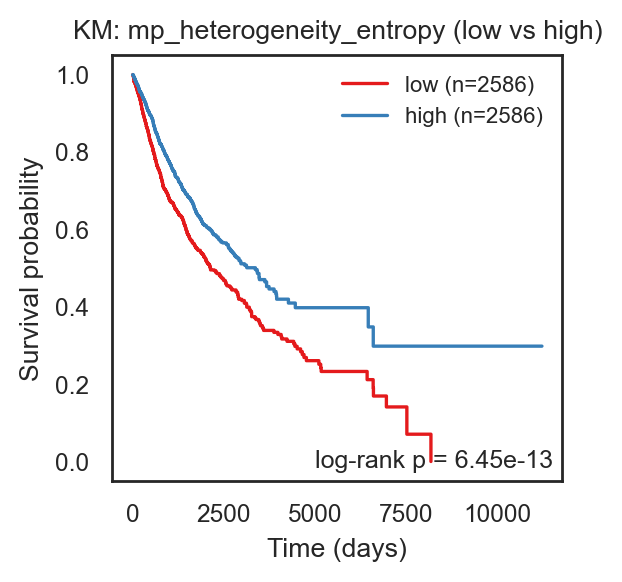
<Axes: title={'center': 'KM: mp_heterogeneity_entropy (low vs high)'}, xlabel='Time (days)', ylabel='Survival probability'>
bk.pl.km_univariate(
adata,
x_key="MKI67",
x_source="gene",
time_key="OS.time",
event_key="OS",
layer="log1p_cpm",
group_col=None,
orce_rebin=True, # if iterating quickly
logrank=True,
figsize=(3, 3),
save="Fig_KM_Heterogeneity_OS.svg",
)
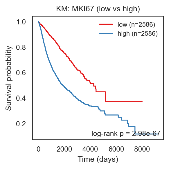
<Axes: title={'center': 'KM: MKI67 (low vs high)'}, xlabel='Time (days)', ylabel='Survival probability'>
bk.pl.km_univariate(
adata,
x_key="Neuroendocrine_score",
time_key="OS.time",
event_key="OS",
logrank=True,
figsize=(3, 3),
save="Fig_KM_Heterogeneity_OS.svg",
)
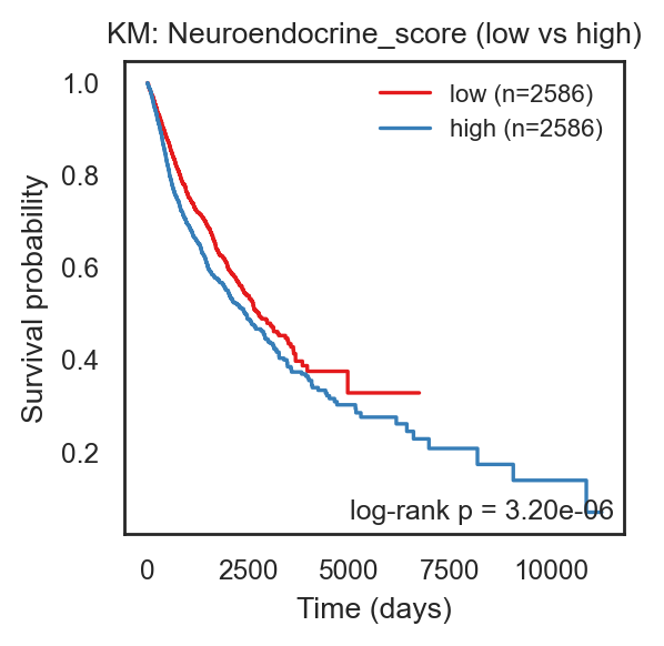
<Axes: title={'center': 'KM: Neuroendocrine_score (low vs high)'}, xlabel='Time (days)', ylabel='Survival probability'>
KM 2x2 interaction#
Cox model stratified by Project_ID (main result)#
Uses lifelines
Term |
Meaning |
|---|---|
NE_bin |
Effect of high vs low NE when heterogeneity is low |
HET_bin |
Effect of high vs low heterogeneity when NE is low |
NE_x_HET |
Extra risk (or protection) when both NE and heterogeneity are high |
If NE_x_HET is significant, that’s your interaction:
NE programs are particularly deleterious in heterogeneous tumors.
bk.pl.km_2x2_interaction(
adata,
x_key="Neuroendocrine_score",
x_source="obs",
z_key="mp_heterogeneity_entropy",
z_source="auto",
layer="log1p_cpm",
group_col=None, # strongly recommended
force_rebin=True,
logrank=True,
figsize=(4,3),
)
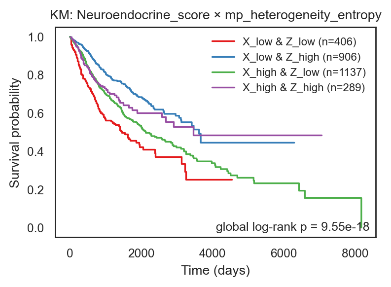
<Axes: title={'center': 'KM: Neuroendocrine_score × mp_heterogeneity_entropy'}, xlabel='Time (days)', ylabel='Survival probability'>
bk.pl.km_2x2_interaction(
adata,
x_key="Proliferation_score",
x_source="obs",
z_key="mp_heterogeneity_entropy",
z_source="auto",
layer="log1p_cpm",
group_col=None, # strongly recommended
force_rebin=True,
logrank=True,
figsize=(4,3),
)
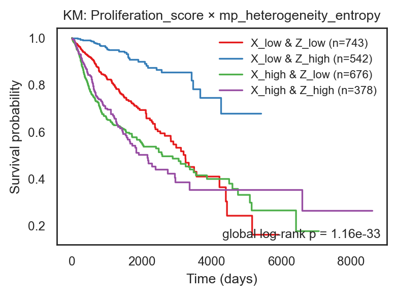
<Axes: title={'center': 'KM: Proliferation_score × mp_heterogeneity_entropy'}, xlabel='Time (days)', ylabel='Survival probability'>
adata_coad = adata[(adata.obs["Project_ID"] == "COAD") | (adata.obs["Project_ID"] == "LUAD")].copy()
bk.pl.km_2x2_interaction(
adata_coad,
x_key="Proliferation_score",
x_source="obs",
z_key="mp_heterogeneity_entropy",
z_source="auto",
min_n=15,
keep="extremes",
layer="log1p_cpm",
group_col=None, # strongly recommended
force_rebin=True,
logrank=True,
figsize=(4,3),
)
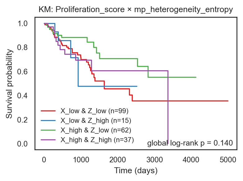
<Axes: title={'center': 'KM: Proliferation_score × mp_heterogeneity_entropy'}, xlabel='Time (days)', ylabel='Survival probability'>
Global quantiles (pan-cancer):
bk.pl.km_2x2_interaction(
adata,
x_key="Neuroendocrine_score", # or "NE25_score"
z_key="mp_heterogeneity_entropy",
x_source="obs", # ["auto", "obs", "gene"] = "auto",
z_source="obs", # ["auto", "obs", "gene"] = "auto",
time_key="OS.time",
event_key="OS",
binning="global", # "global" | "within_group"
logrank=True,
q=(0.25, 0.75),
min_n=50,
figsize=(3, 3),
save="Fig_KM_NE_x_Heterogeneity.svg",
)
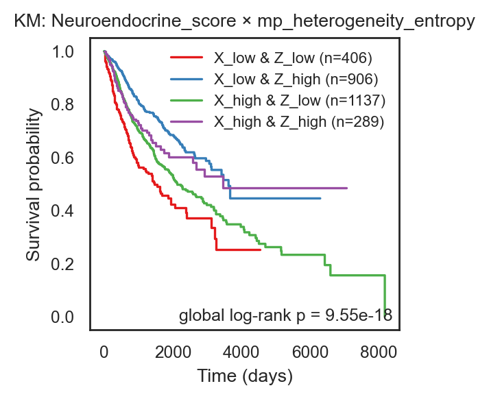
<Axes: title={'center': 'KM: Neuroendocrine_score × mp_heterogeneity_entropy'}, xlabel='Time (days)', ylabel='Survival probability'>
bk.pl.km_2x2_interaction(
adata,
x_key="Proliferation_score", # or "NE25_score"
z_key="mp_heterogeneity_entropy",
time_key="OS.time",
event_key="OS",
binning="global",
logrank=True,
q=(0.25, 0.75),
min_n=50,
figsize=(3, 3),
save="Fig_KM_NE_x_Heterogeneity.svg",
)
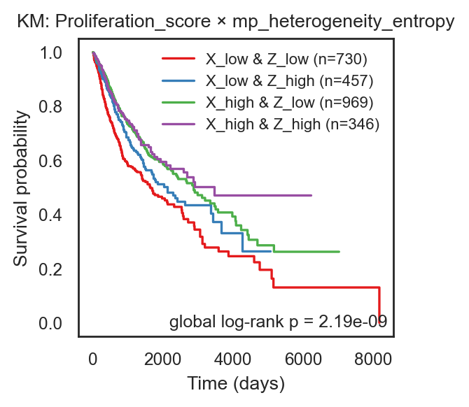
<Axes: title={'center': 'KM: Proliferation_score × mp_heterogeneity_entropy'}, xlabel='Time (days)', ylabel='Survival probability'>
Within tumor type quantiles (optional, often fairer):
bk.pl.km_2x2_interaction(
adata,
x_key="Neuroendocrine_score",
z_key="mp_heterogeneity_entropy",
time_key="OS.time",
event_key="OS",
binning="within_group",
groupby_for_binning="Project_ID",
logrank=True,
q=(0.25, 0.75),
min_n=40,
figsize=(3, 3),
save=DESKTOP+"Fig_KM_NE_x_Heterogeneity_withinTumor.svg",
)
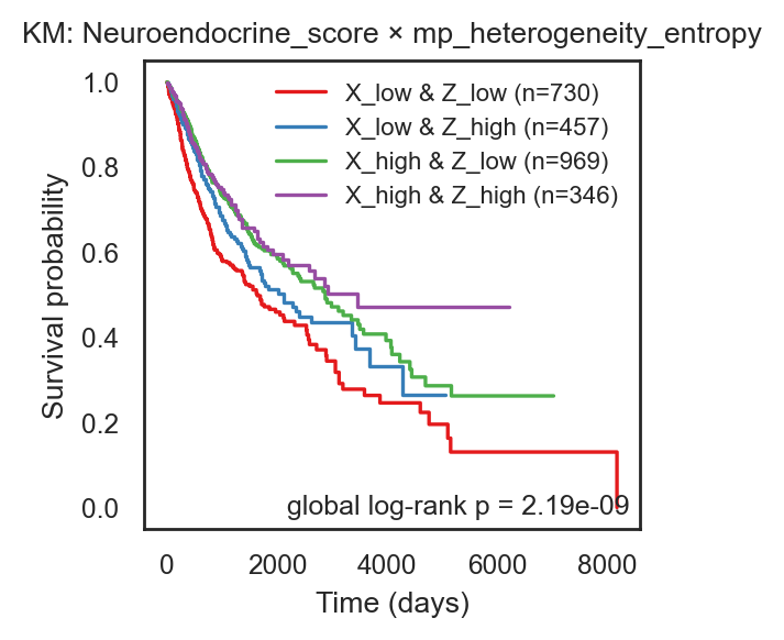
<Axes: title={'center': 'KM: Neuroendocrine_score × mp_heterogeneity_entropy'}, xlabel='Time (days)', ylabel='Survival probability'>
Use it also for interaction between genes
bk.pl.km_2x2_interaction(
adata,
x_key="MYC",
x_source="gene",
z_key="RB1_mut",
z_source="obs",
layer="log1p_cpm",
group_col=None, # strongly recommended
force_rebin=True,
logrank=True,
figsize=(4,3),
)
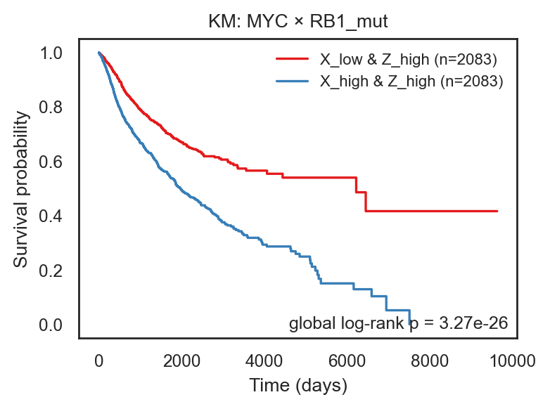
<Axes: title={'center': 'KM: MYC × RB1_mut'}, xlabel='Time (days)', ylabel='Survival probability'>
bk.pl.km_2x2_interaction(
adata,
x_key="MYC",
x_source="gene",
z_key="CCNE1",
z_source="gene",
layer="log1p_cpm",
group_col=None, # strongly recommended
force_rebin=True,
logrank=True,
figsize=(4,3),
)
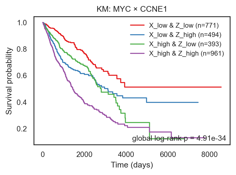
<Axes: title={'center': 'KM: MYC × CCNE1'}, xlabel='Time (days)', ylabel='Survival probability'>
You can easily extend the model:
formula = "NE_bin + HET_bin + NE_x_HET + age + gender"
Change palette in km_2x2:
bk.pl.km_2x2_interaction(
adata,
x_key="RB1_mut",
x_source="obs",
x_binary_mode="auto",
x_binary_labels=("WT","Mut"),
z_key="mp_heterogeneity_entropy",
z_source="obs",
palette={
"X_low & Z_low": "tab:blue",
"X_low & Z_high": "tab:cyan",
"X_high & Z_low": "tab:orange",
"X_high & Z_high": "tab:red",
},
min_n=30,
logrank=True,
force_rebin=True,
)
bk.pl.km_2x2_interaction(
adata,
palette=("tab:blue", "tab:green", "tab:orange", "tab:red"),
)
12. General Plots#
12.1. Dotplot#
# Check if genes have zeros (e.g. Fraction of samples expressing is not 1)
genes = ["CDK1","MKI67","CD3E","CD79A","MS4A1"]
gidx = [adata.var_names.get_loc(g) for g in genes]
X = adata.layers["counts"][:, gidx]
X = X.toarray() if hasattr(X, "toarray") else np.asarray(X)
print("fraction >0 per gene:", (X > 0).mean(axis=0))
print("min/max counts per gene:", X.min(axis=0), X.max(axis=0))
fraction >0 per gene: [1. 1. 0.98876404 0.88764045 0.88764045]
min/max counts per gene: [5 2 0 0 0] [1156 1003 195 383 966]
bk.pl.dotplot(
adata,
var_names=["CDK1","MKI67","CD3E","CD79A","MS4A1"],
groupby="Subtype_PAM50",
swap_axes=True,
row_spacing = 0.4,
dendrogram_top=True,
dendrogram_rows=True,
row_dendrogram_position="outer_left",
title=None,
)
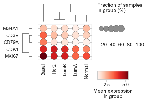
(<Figure size 615x475 with 5 Axes>, <Axes: >)
markers = {
"B-cell": ["CD79A","MS4A1"],
"Dendritic": ["FCER1A"],
"Monocytes": ["CST3","FCGR3A"],
"NK": ["GNLY","NKG7"],
"Other": ["IGLL1"],
"T-cell": ["CD3D"],
}
#var_groups dict (Scanpy-like brackets + ordering)
bk.pl.dotplot(
adata,
var_groups=markers,
groupby="Subtype_PAM50",
swap_axes=False,
row_spacing = 0.4,
dendrogram_rows=True, # cluster groups
dendrogram_top=True, # cluster genes within the full list (still keeps brackets)
save="figs/dotplot_scanpy_like.png",
)
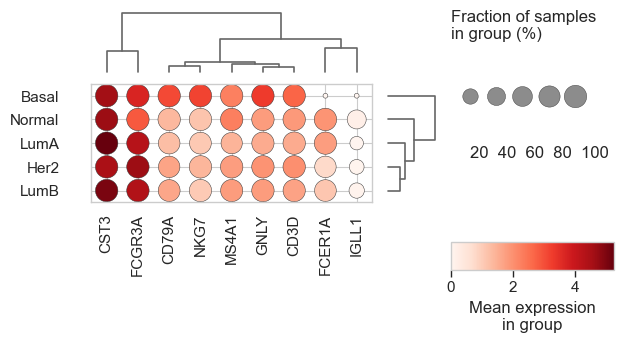
(<Figure size 835x475 with 5 Axes>, <Axes: >)
CHECK MARKERS DICT GROUPS WITH NO DENDRIMGRAM#
bk.pl.dotplot(
adata,
var_groups=markers,
groupby="Subtype_PAM50",
swap_axes=False,
row_spacing = 0.4,
dendrogram_rows=True, # cluster groups
dendrogram_top=False, # cluster genes within the full list (still keeps brackets)
save="figs/dotplot_scanpy_like.png",
)
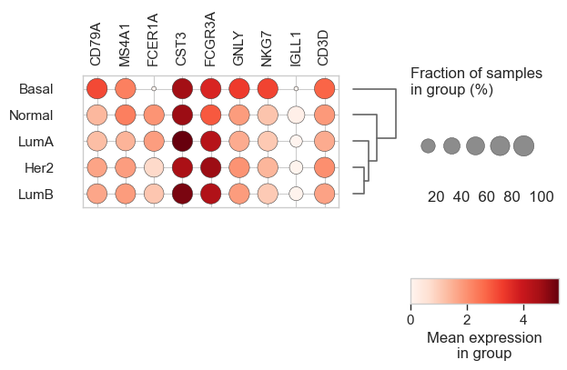
(<Figure size 835x475 with 4 Axes>, <Axes: >)
12.2. Heatmap#
res.columns.tolist()
['gene', 'log2FC', 't', 'pval', 'qval', 'mean_group', 'mean_ref']
# 2) heatmap of top DE genes
bk.pl.heatmap_de(
adata,
contrast="LumB_vs_LumA",
groupby="Subtype_PAM50",
groups=["LumA", "LumB"],
layer="log1p_cpm",
top_n=60,
mode="both",
col_colors=["Subtype_PAM50"],
save=DESKTOP + "clustermap.png",
)
---------------------------------------------------------------------------
KeyError Traceback (most recent call last)
File ~/Library/CloudStorage/OneDrive-VHIO/BioInformatics/BioProjects/MM01_BULLKpy/bullkpy-skeleton/src/bullkpy/pl/heatmap_de.py:74, in heatmap_de(adata, contrast, de_key, results_key, layer, groupby, groups, top_n, mode, sort_by, z_score, clip_z, cmap, center, col_colors, dendrogram_rows, dendrogram_cols, show_sample_labels, figsize, cbar_label, save, show)
73 try:
---> 74 res = adata.uns[de_key][contrast][results_key]
75 except KeyError as e:
KeyError: 'de'
The above exception was the direct cause of the following exception:
KeyError Traceback (most recent call last)
Cell In[51], line 2
1 # 2) heatmap of top DE genes
----> 2 bk.pl.heatmap_de(
3 adata,
4 contrast="LumB_vs_LumA",
5 groupby="Subtype_PAM50",
6 groups=["LumA", "LumB"],
7 layer="log1p_cpm",
8 top_n=60,
9 mode="both",
10 col_colors=["Subtype_PAM50"],
11 save=DESKTOP + "clustermap.png",
12 )
File ~/Library/CloudStorage/OneDrive-VHIO/BioInformatics/BioProjects/MM01_BULLKpy/bullkpy-skeleton/src/bullkpy/pl/heatmap_de.py:76, in heatmap_de(adata, contrast, de_key, results_key, layer, groupby, groups, top_n, mode, sort_by, z_score, clip_z, cmap, center, col_colors, dendrogram_rows, dendrogram_cols, show_sample_labels, figsize, cbar_label, save, show)
74 res = adata.uns[de_key][contrast][results_key]
75 except KeyError as e:
---> 76 raise KeyError(
77 f"Could not find DE results at adata.uns['{de_key}']['{contrast}']['{results_key}']"
78 ) from e
80 if not isinstance(res, pd.DataFrame):
81 res = pd.DataFrame(res)
KeyError: "Could not find DE results at adata.uns['de']['LumB_vs_LumA']['results']"
12.3. Violin plot#
bk.pl.violin(
adata,
keys=["total_counts", "pct_counts_mt", "n_genes_detected"],
groupby="Subtype_PAM50",
order=["LumA", "LumB", "Her2", "Basal", "Normal"],
#figsize=(6, 3),
save="figs/violin_qc.png",
)
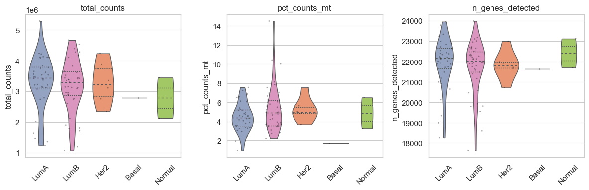
(<Figure size 1200x400 with 3 Axes>,
array([<Axes: title={'center': 'total_counts'}, ylabel='total_counts'>,
<Axes: title={'center': 'pct_counts_mt'}, ylabel='pct_counts_mt'>,
<Axes: title={'center': 'n_genes_detected'}, ylabel='n_genes_detected'>],
dtype=object))
bk.pl.violin_genes(adata, genes=["MKI67","E2F1", "TPX2"], groupby="Subtype_PAM50",
order=["LumA", "LumB", "Her2", "Basal", "Normal"],
layer="log1p_cpm",
#figsize=(3, 4),
save="figs/violin_genes.png")
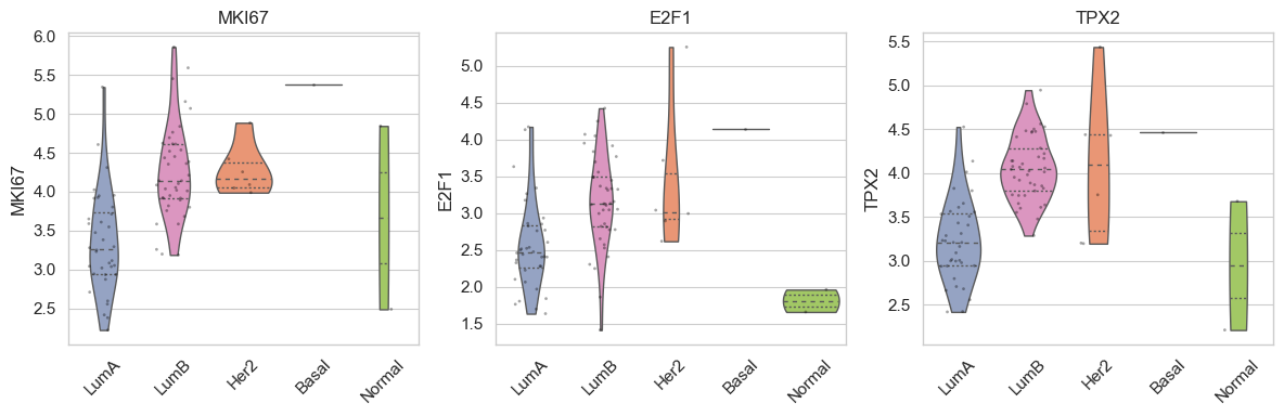
(<Figure size 1200x400 with 3 Axes>,
array([<Axes: title={'center': 'MKI67'}, ylabel='MKI67'>,
<Axes: title={'center': 'E2F1'}, ylabel='E2F1'>,
<Axes: title={'center': 'TPX2'}, ylabel='TPX2'>], dtype=object))
12.4. Violin Gene Plot#
bk.pl.gene_plot(
adata_lung,
gene="MKI67",
groupby="Project_ID",
layer="log1p_cpm",
test="auto", # defaults to Kruskal
kind="both",
figsize=(2.5,3),
save=DESKTOP + "MKI67_by_lung.png",
)
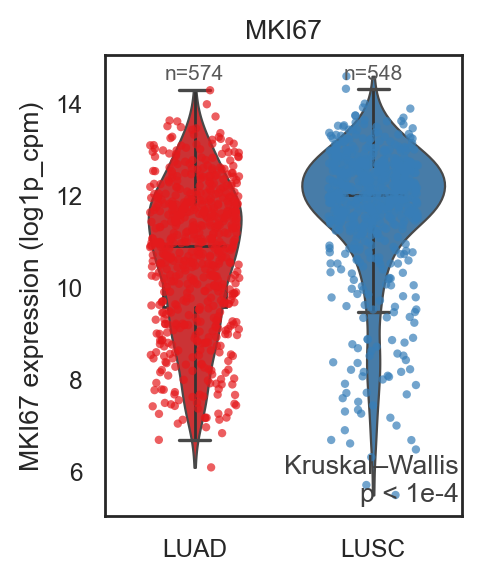
(<Figure size 500x600 with 1 Axes>,
<Axes: title={'center': 'MKI67'}, ylabel='MKI67 expression (log1p_cpm)'>,
{'test': 'Kruskal–Wallis', 'pvalue': 9.651818201137253e-34, 'compare': None})
bk.pl.gene_plot(
adata,
gene="MKI67",
groupby="Project_ID",
layer="log1p_cpm",
test="auto", # defaults to Kruskal
kind="both",
figsize=(7,3),
save=DESKTOP + "MKI67_by_lung.png",
)
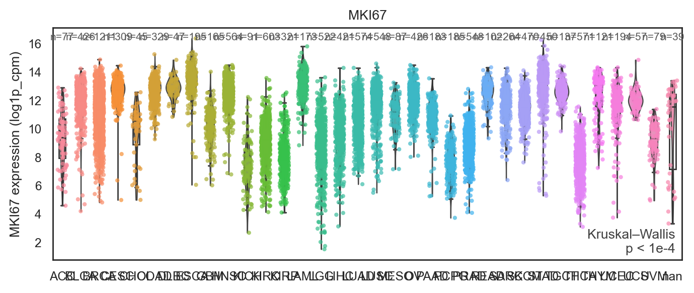
(<Figure size 1400x600 with 1 Axes>,
<Axes: title={'center': 'MKI67'}, ylabel='MKI67 expression (log1p_cpm)'>,
{'test': 'Kruskal–Wallis', 'pvalue': 0.0, 'compare': None})
# Overall p-value across all PAM50 subtypes
bk.pl.gene_plot(
adata,
gene="CDK1",
groupby="Subtype_PAM50",
layer="log1p_cpm",
test="auto", # defaults to Kruskal
kind="both",
figsize=(4,4),
save="figs/CDK1_by_PAM50.png",
)
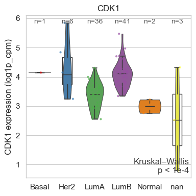
(<Figure size 400x400 with 1 Axes>,
<Axes: title={'center': 'CDK1'}, ylabel='CDK1 expression (log1p_cpm)'>,
{'test': 'Kruskal–Wallis', 'pvalue': 3.3816506907753345e-07, 'compare': None})
# Pairwise LumA vs LumB with bracket
bk.pl.gene_plot(
adata,
gene="MKI67",
groupby="Subtype_PAM50",
layer="log1p_cpm",
compare=["LumA", "LumB"],
test="wilcoxon", # Mann–Whitney U
kind="both",
figsize=(5,4),
save="figs/MKI67_LumA_vs_LumB.png",
)
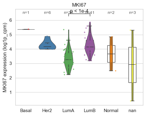
(<Figure size 500x400 with 1 Axes>,
<Axes: title={'center': 'MKI67'}, ylabel='MKI67 expression (log1p_cpm)'>,
{'test': 'Mann–Whitney U',
'pvalue': 5.433595540609767e-08,
'compare': ['LumA', 'LumB']})
12.5. Sample distances#
A) Sample distances (Euclidean on log1p_cpm) + metadata colors
bk.pl.sample_distances(
adata,
layer="log1p_cpm",
metric="euclidean",
method="average",
col_colors=["Subtype_PAM50", "Batch"],
show_labels=False,
save="figs/sample_distances.png",
)
B) Sample correlation clustergram (recommended for bulk QC)
bk.pl.sample_correlation_clustergram(
adata,
layer="log1p_cpm",
method="pearson",
col_colors=["Subtype_PAM50", "Batch"],
show_labels=False,
save="figs/sample_corr_clustergram.png",
)
C) Spearman correlation version (robust)
bk.pl.sample_correlation_clustergram(
adata,
layer="log1p_cpm",
method="spearman",
col_colors=["Subtype_PAM50"],
save="figs/sample_corr_spearman.png",
)
12.6. Oncoprint#
bk.pl.oncoprint(
adata_lung,
mut_cols=["KRAS_mut", "TP53_mut", "RB1_mut", "STK11_mut", "KEAP1_mut"],
groupby="Project_ID",
group_blocks=True,
grid_color="0.9",
title=None,
fontsize=12,
#figsize=(15,2),
save=DESKTOP + "oncoprint_mutfirst_by_project.png",
)
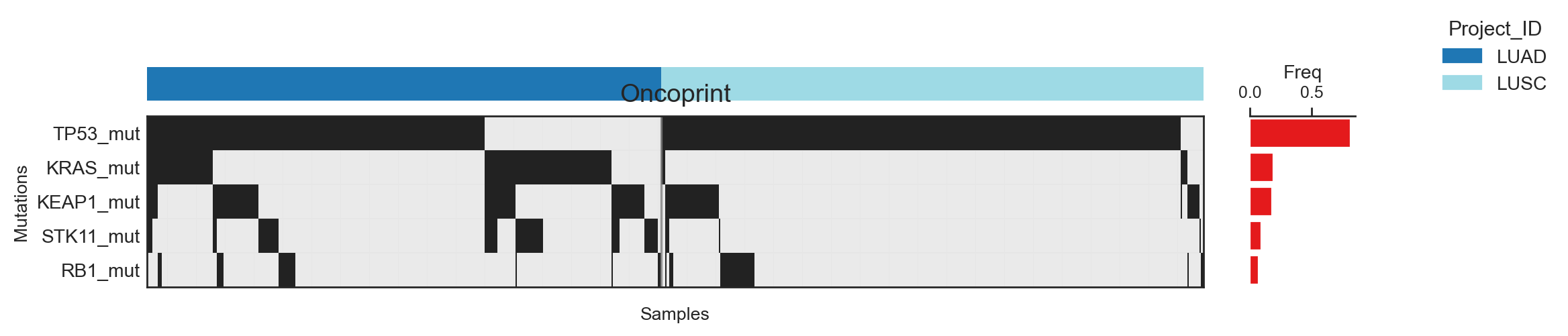
(<Figure size 3000x400 with 3 Axes>,
<Axes: title={'center': 'Oncoprint'}, xlabel='Samples', ylabel='Mutations'>)
bk.pl.oncoprint(
adata_lung,
mut_cols=["KRAS_mut", "TP53_mut", "RB1_mut", "STK11_mut", "KEAP1_mut"],
groupby="Project_ID",
group_blocks=True,
fontsize=20,
title=" ",
figsize=(20,3),
save=DESKTOP + "oncoprint_mutfirst_by_project_lung.png",
)
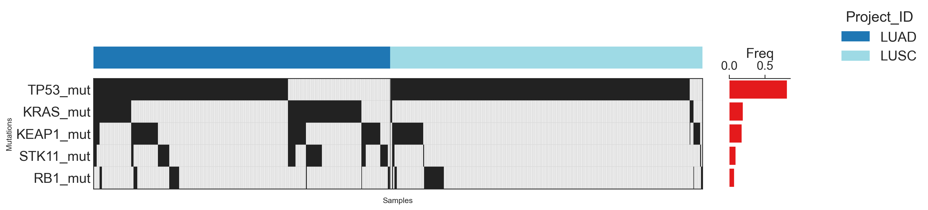
(<Figure size 4000x600 with 3 Axes>,
<Axes: title={'center': ' '}, xlabel='Samples', ylabel='Mutations'>)
# Large datasets (avoid huge images)
bk.pl.oncoprint(
adata,
mut_cols=["KRAS_mut", "TP53_mut", "RB1_mut", "STK11_mut", "KEAP1_mut"],
groupby="Project_ID",
max_samples=800, # IMPORTANT for TCGA-scale
cell_size=0.03, # compact columns
fontsize=20,
title=" ",
save_dpi=300, # keep under pixel limit
save=DESKTOP + "oncoprint_big.png",
)
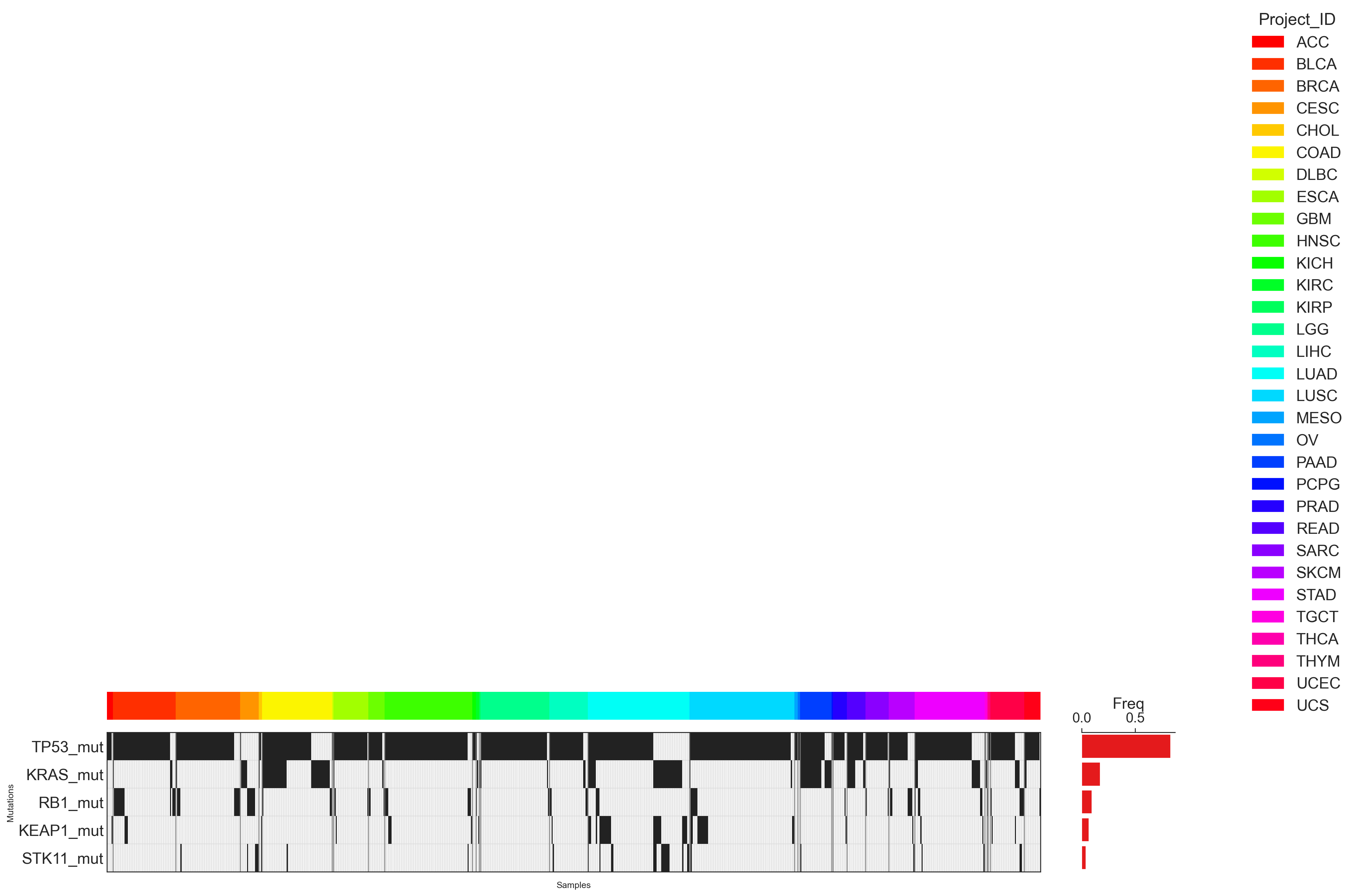
(<Figure size 5360x660 with 3 Axes>,
<Axes: title={'center': ' '}, xlabel='Samples', ylabel='Mutations'>)
#Add expression tracks under the mutations
bk.pl.oncoprint(
adata_lung,
mut_cols=["RB1_mut", "TP53_mut", "KEAP1_mut", "STK11_mut"],
expr_genes=["DLL3", "ASCL1", "SOX2", "MKI67"],
layer="log1p_cpm",
expr_zscore=True, # makes expression rows comparable
groupby="Project_ID",
sort_samples="pattern",
#top_annotation_height=0.35,
title=" ",
fontsize=24,
save_dpi=300,
save=DESKTOP + "oncoprint_plus_expr.png",
)
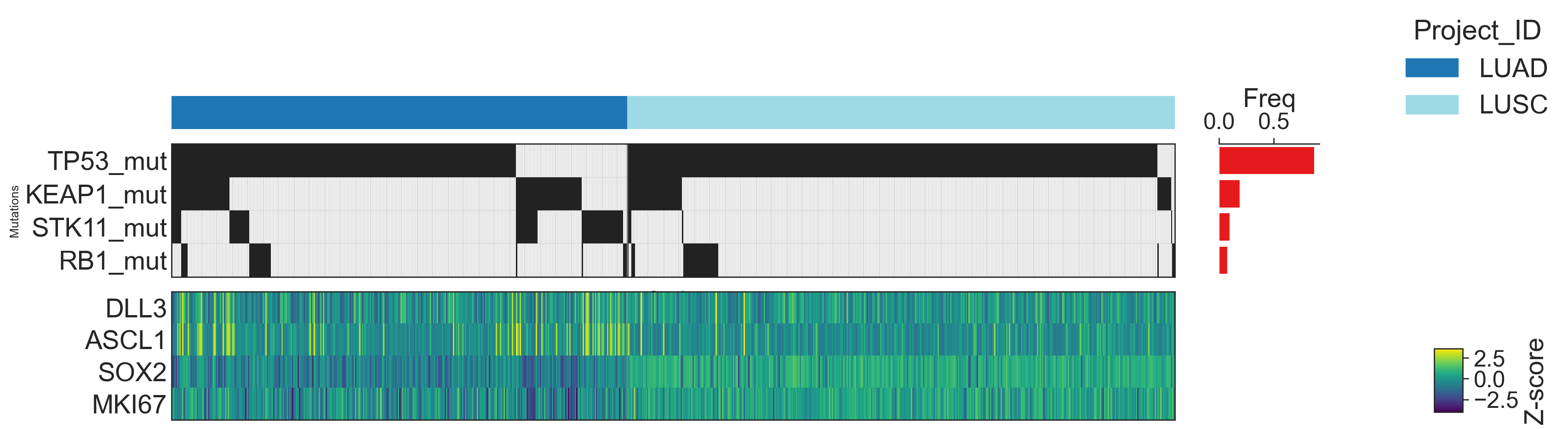
(<Figure size 4160x860 with 5 Axes>,
<Axes: title={'center': ' '}, xlabel='Samples', ylabel='Mutations'>)
# Control the order
bk.pl.oncoprint(
adata_lung,
drop_all_wt = False,
mut_cols=["RB1_mut", "TP53_mut"],
#group_order=, # or any subset/order list(adata.obs_names),
sort_samples="mut_first" # "burden", #"none",
)
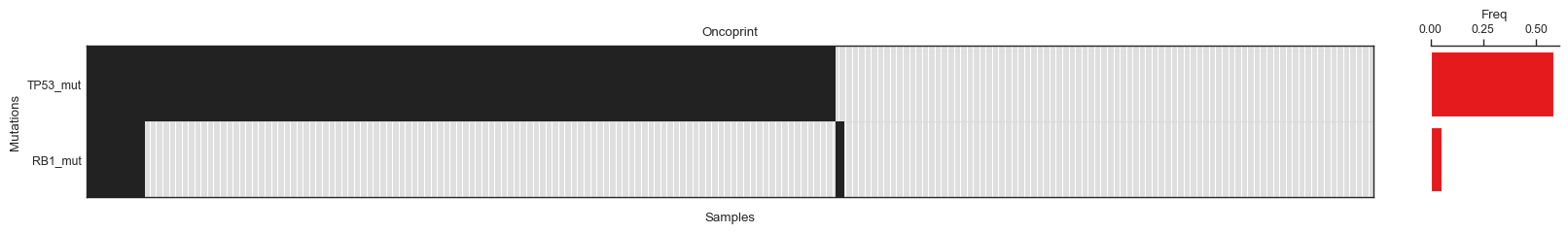
(<Figure size 2524x190 with 2 Axes>,
<Axes: title={'center': 'Oncoprint'}, xlabel='Samples', ylabel='Mutations'>)
13. Utilities#
13.1. Pandas for manipulating expression data and metadata#
Set Sample ID as index using pandas and transpose the table
13.2 Sanitize metadata#
OPTIONAL.
It is important that metadata columns are in the proper dtype (categories, numeric, text, etc.) for downstream studies. IF you get problems later with your metadata you can use this utilite below
Check observations
bad, _ = bk.pp.find_bad_obs_cols_by_write(adata, n_rows=3000)
print("bad before:", len(bad), bad[:10])
print(" --------------------- ")
adata_safe, rep = bk.pp.make_obs_h5ad_safe_strict(adata, copy=True)
print(rep)
print(" --------------------- ")
bad2, _ = bk.pp.find_bad_obs_cols_by_write(adata_safe, n_rows=3000)
print("bad after (2nd):", len(bad2), bad2[:10])
bad before: 0 []
---------------------
{'numeric_coerced': [], 'string_to_object': [], 'stringified': [], 'category_fixed': [], 'errors': []}
---------------------
bad after (2nd): 0 []
Check var
adata_safe.var_names_make_unique() # recommended
_, rep_var = bk.pp.make_var_h5ad_safe_strict(adata_safe, copy=False)
print(rep_var)
# re-test var
bad_var2, _ = bk.pp.find_bad_var_cols_by_write(adata_safe, n_cols=60000)
print("bad var after:", len(bad_var2), bad_var2[:20])
{'string_to_object': [], 'category_fixed': [], 'bytes_stringified': [], 'nonscalar_stringified': [], 'mixed_object_stringified': ['Chromosome/scaffold name'], 'errors': [], 'n_cols': 14}
bad var after: 0 []
Once bad/bad var == 0:
adata = adata_safe.copy()
adata.write("../data/h5ad/260127_TCGA_example_in_BULLKpy.h5ad", compression="gzip")
13.3. Batch Correction#
Best practice is to run ComBat on log-normalized expression (not raw counts):
adata.obs.Batch.value_counts()
Batch4 29
Batch2 17
Batch3 17
Batch1 13
Batch5 10
Name: Batch, dtype: int64
bk.pp.batch_correct_combat(
adata,
batch_key="Batch",
layer="log1p_cpm",
covariates=["Subtype_PAM50"], # preserve biology
key_added="combat_log1p_cpm",
)
adata.layers
Layers with keys: counts, cpm, log1p_cpm, combat_log1p_cpm
#then use downstream
bk.tl.pca(adata, layer="combat_log1p_cpm", use_highly_variable=True)
bk.tl.neighbors(adata, use_rep="X_pca", n_neighbors=15)
bk.tl.umap(adata)