GSEA bubbleplot#
- bullkpy.pl.gsea_bubbleplot(df_gsea, *, pathways, comparison_col='comparison', term_col='Term', nes_col='NES', fdr_col='FDR q-val', comparison_order=None, drop_empty_comparisons=True, size_from='fdr', min_q=1e-300, size_min=10.0, size_max=350.0, fdr_floor=1e-50, size_clip_quantile=0.99, cmap='RdBu_r', center=0.0, vmin=None, vmax=None, figsize=None, row_spacing=1.0, col_spacing=1.0, row_height=0.32, col_width=0.32, dot_edgecolor='0.15', dot_linewidth=0.35, show_grid=False, group_label_rotation=90, xtick_rotation=90, title=None, save=None, show=True)[source]#
Bubble plot matrix for GSEA results.
Rows: comparisons (contrasts) Cols: pathways (terms) Color: NES (diverging, centered at center) Size: -log10(FDR q-val) with floor & optional clipping
- pathways can be:
dict: {“Immune”: [term1, term2], “Metabolism”: [term3]}
list: [term1, term2, …]
Bubble-plot matrix for GSEA results across multiple comparisons (contrasts).
Each dot encodes enrichment direction/strength and significance for a given (comparison × pathway).
Rows: comparisons (e.g., contrasts like
"Basal_vs_Luminal")Columns: pathways/terms (e.g., Hallmark sets)
Color:
NES(diverging colormap, centered atcenter)Size:
-log10(FDR q-val)with a floor and optional clipping
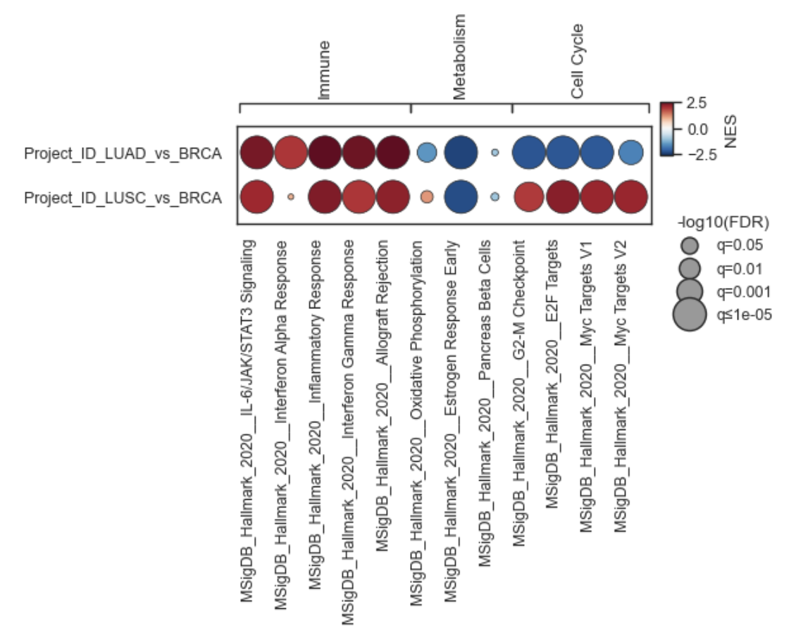
Example GSEA bubble plot
Expected input#
df_gsea
A tidy GSEA results table (often concatenated across contrasts), containing at least:
comparison_col (default: “comparison”)
term_col (default: “Term”)
nes_col (default: “NES”)
fdr_col (default: “FDR q-val”)
If any are missing, the function raises a KeyError.
pathways
Selects which terms to display, and optionally groups them for visual brackets.
Accepted forms:
Mapping (grouped columns with brackets):
pathways = {
  "Immune": ["HALLMARK_INTERFERON_GAMMA_RESPONSE", "HALLMARK_INFLAMMATORY_RESPONSE"],
  "Cell cycle": ["HALLMARK_E2F_TARGETS", "HALLMARK_G2M_CHECKPOINT"],
}
Sequence (flat list of terms):
pathways = ["HALLMARK_E2F_TARGETS", "HALLMARK_P53_PATHWAY"]
What it does#
Validates columns in df_gsea.
Flattens pathways.
If a dict is provided, it preserves group spans so it can draw bracket labels above term blocks.
Produces: – terms: ordered list of pathways to plot – spans: (start, end, group_label) intervals (dict mode only).
Subsets results. Keeps only rows where term_col is in the requested terms.
Builds matrices.
nes_mat: pivot of NES (rows=comparisons, cols=terms)
q_mat: pivot of FDR q-values (rows=comparisons, cols=terms)
Aggregation uses mean if duplicate rows exist for a cell.
Orders comparisons
If comparison_order is provided, uses it.
Otherwise uses categorical order if available, else sorted unique comparisons.
Optionally drops empty comparisons
If drop_empty_comparisons=True, removes rows where all selected terms are missing.Maps dot size from significance.
Converts q-values to size_signal = -log10(q)
loors q-values: – Non-finite → NaN – q <= 0 → fdr_floor – Clamp q to [fdr_floor, 1.0]
Optional clipping: If size_clip_quantile is not None, caps size_signal at that quantile to prevent a few tiny q-values dominating dot sizes.
Rescales linearly to [size_min, size_max].
If NES is missing for a cell → dot size is set to 0 (not drawn).
Maps dot color from NES.
Uses a single TwoSlopeNorm(vcenter=center) so: Negative NES and positive NES are visually balanced around center.
If vmin/vmax not provided, bounds are set symmetrically using the max absolute NES observed.
Plots.
One scatter call for all dots (ensures the colorbar matches the dots).
Y-axis is inverted (Scanpy-like).
Optional grid.
Adds legends
Colorbar labeled “NES”.
Size legend labeled “-log10(FDR)” using reference q-values (e.g. 0.05, 0.01, 0.001, and the floor).
Optionally saves If save is provided, uses _savefig(fig, save).
Parameters#
Required#
df_gsea: DataFrame of GSEA results
pathways: terms (list) or grouped terms (dict)
Column mapping#
comparison_col: column identifying contrasts (default “comparison”)
term_col: pathway/term name column (default “Term”)
nes_col: NES column (default “NES”)
fdr_col: FDR q-value column (default “FDR q-val”)
Ordering#
comparison_order: explicit ordering for rows
drop_empty_comparisons: drop comparisons with no selected terms
Size mapping (significance → bubble area)#
size_from: currently intended “fdr” (q-values); kept for future flexibility
dr_floor: smallest q-value used for size computation (prevents -log10(0))
size_clip_quantile: cap size signal at a quantile (default 0.99)
size_min / size_max: dot size range (in matplotlib “area” units)
Color mapping (NES → color)#
cmap: diverging colormap (default “RdBu_r”)
center: value treated as neutral (default 0.0)
vmin / vmax: optional explicit NES bounds
Layout / cosmetics#
figsize: if None, chosen from number of rows/cols using row_height and col_width -row_spacing / col_spacing: spacing between dot centers
dot_edgecolor / dot_linewidth: dot outline styling
show_grid: toggle grid
group_label_rotation: rotation for pathway group labels (dict mode)
xtick_rotation: rotation for pathway labels
title: plot title
Output#
save: path to save figure
show: whether to display via plt.show()
Returns#
(fig, ax): Matplotlib Figure and Axes.
Notes / tips#
Use grouped pathways (dict) when you want to visually separate pathway themes.
If you see extremely large dots overwhelming the plot, lower size_clip_quantile (e.g. 0.95) or increase fdr_floor.
If NES ranges differ greatly across runs and you want consistent scaling across figures, pass fixed vmin and vmax.
Examples#
Basic bubble plot for a fixed set of terms
fig, ax = bk.pl.gsea_bubbleplot(
    df_gsea,
    pathways=[
        "HALLMARK_E2F_TARGETS",
        "HALLMARK_G2M_CHECKPOINT",
        "HALLMARK_P53_PATHWAY",
    ],
)
Grouped pathways + custom comparison order
pathways = {
    "Cell cycle": ["HALLMARK_E2F_TARGETS", "HALLMARK_G2M_CHECKPOINT"],
    "Immune": ["HALLMARK_INTERFERON_GAMMA_RESPONSE", "HALLMARK_INFLAMMATORY_RESPONSE"],
}

fig, ax = bk.pl.gsea_bubbleplot(
    df_gsea,
    pathways=pathways,
    comparison_order=["Basal_vs_rest", "Luminal_vs_rest", "Her2_vs_rest"],
    size_clip_quantile=0.98,
    title="Hallmark GSEA summary",
)