ARI resolution heatmap#
- bullkpy.pl.ari_resolution_heatmap(adata, *, df=None, store_key='leiden_scan', metric='ARI', show_n_clusters=True, cmap='viridis', vmin=None, vmax=None, figsize=None, title=None, save=None, show=True)[source]#
Heatmap-like summary of clustering quality vs Leiden resolution.
- Expects df with at least:
‘resolution’
metric column: ‘ARI’ or ‘NMI’ or ‘cramers_v’
- Optional:
‘n_clusters’ (for a second row annotation)
Example
df = bk.tl.leiden_resolution_scan(…) bk.pl.ari_resolution_heatmap(adata, df=df, metric=”ARI”)
Heatmap-style summary of clustering quality across Leiden resolutions.
This function visualizes the output of a Leiden resolution scan
(e.g. from bk.tl.leiden_resolution_scan) and helps identify
stable or optimal resolutions based on clustering quality metrics.
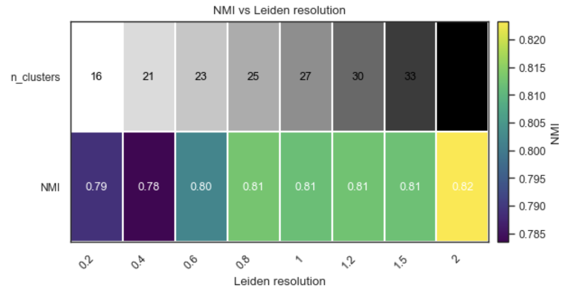
Example ARI resolution heatmap
What it does#
Displays clustering quality (e.g. ARI, NMI, or Cramér’s V) as a single-row heatmap across Leiden resolutions.
Optionally adds a second row showing the number of clusters
Annotates each cell with the metric value (and cluster count)
Designed to be compact, readable, and Scanpy-like.
This plot is ideal for resolution selection and reporting.
Expected input#
The function expects a DataFrame (either passed directly or stored in adata.uns) with at least:
column |
description |
|---|---|
resolution |
Leiden resolution values |
ARI / NMI / cramers_v |
clustering quality metric |
Optional:
column |
description |
|---|---|
n_clusters |
number of clusters at each resolution |
Such a table is produced by:
bk.tl.leiden_resolution_scan(adata, true_key=...)
Parameters#
adata
AnnData object. Used to retrieve results from adata.uns
if df is not provided.
df
DataFrame with resolution scan results.
If None, adata.uns[store_key] is used.
store_key
Key in adata.uns where resolution scan results are stored
(default: “leiden_scan”).
metric
Clustering quality metric to visualize.
Supported values:
“ARI”
“NMI”
“cramers_v”
show_n_clusters
If True and n_clusters is present, adds a second row
showing the number of clusters.
cmap
Colormap for the metric heatmap.
vmin, vmax
Optional color scale limits for the metric.
figsize
Figure size in inches.
If None, a sensible size is inferred from the number of resolutions.
title
Optional plot title.
save
Path to save the figure (PDF/PNG/SVG).
show
Whether to immediately display the plot.
Returns#
(fig, ax)
fig: matplotlib Figure.
ax: matplotlib Axes.
Examples#
Basic ARI vs resolution plot
df = bk.tl.leiden_resolution_scan(
    adata,
    true_key="cell_type",
)

bk.pl.ari_resolution_heatmap(
    adata,
    df=df,
    metric="ARI",
)
Include number of clusters
bk.pl.ari_resolution_heatmap(
    adata,
    metric="ARI",
    show_n_clusters=True,
    title="Leiden resolution scan",
)
Use a different metric (Cramér’s V)
bk.pl.ari_resolution_heatmap(
    adata,
    metric="cramers_v",
    cmap="magma",
)
Fix color scale and save figure
bk.pl.ari_resolution_heatmap(
    adata,
    metric="ARI",
    vmin=0,
    vmax=1,
    save="leiden_resolution_ari.png",
)
Notes#
This function does not recompute clustering; it only visualizes results.
Designed for bulk and pseudobulk workflows, but works for single-cell too.
If sklearn was not available during the scan, ARI/NMI values may be NaN (Cramér’s V is always computed).
See also#
•	tl.leiden_resolution_scan
•	tl.cluster
•	pl.plot_corr_heatmap