QC metrics#
- bullkpy.pl.qc_metrics(adata, *, color='pct_counts_mt', vars_to_plot=('total_counts', 'n_genes_detected', 'pct_counts_mt', 'pct_counts_ribo'), log1p_total_counts=True, log1p_n_genes=False, point_size=20.0, alpha=0.8, figsize=(10, 7), save=None, show=True)[source]#
Plot bulk RNA-seq QC metrics (robust to missing columns).
If total_counts + n_genes_detected exist: scatter (library size vs detected genes)
Otherwise: skip scatter and show histograms only
Plot a compact set of bulk RNA-seq QC diagnostics from columns in adata.obs.
The function is robust to missing QC columns: it will plot what is available and warn
about missing variables.
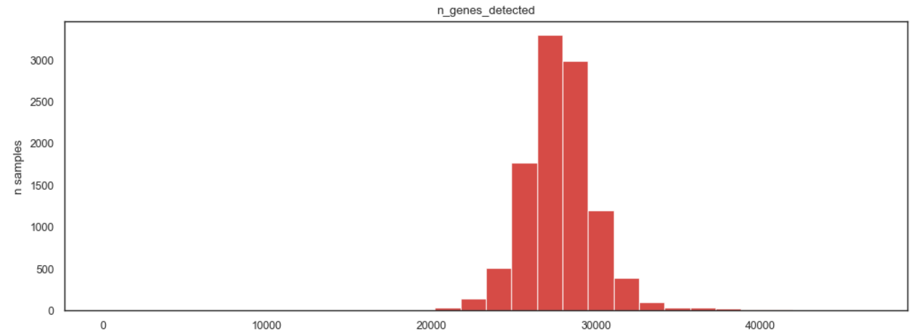
Example QC metrics plot
What it does.#
Depending on what exists in adata.obs, this function produces:
Scatter plot (if possible): library size vs detected genes.
x: total_counts (optionally log1p)
y: n_genes_detected (optionally log1p)
optional point coloring by an obs column (color=).
** 2. Histograms (always, if variables exist): Up to four QC distributions from vars_to_plot:
histogram of the 1st variable (vars_use[0])
histogram of the 2nd variable (vars_use[1])
optional overlay histogram of the 3rd variable on the first histogram (twin y-axis)
optional overlay histogram of the 4th variable on the second histogram (twin y-axis).
If either total_counts or n_genes_detected is missing, the scatter is skipped and only histograms are shown.
Requirements#
adata.obs must contain at least one of the entries in vars_to_plot.
For the scatter panel, adata.obs must include both:
total_counts
n_genes_detected.
If none of vars_to_plot exists, the function raises a KeyError with a suggestion to run a QC computation step first (e.g., bk.pp.qc_metrics).
Parameters#
Core inputs#
adata (anndata.AnnData). Annotated data matrix with QC metrics stored in adata.obs.
Plot selection#
vars_to_plot (Sequence[str]). Ordered list of QC columns to try plotting. The function will use only those that actually exist in adata.obs, in the same order.
Coloring#
color (str | None, default “pct_counts_mt”). Optional adata.obs column used to color points in the scatter plot.
If missing, coloring is disabled with a warning.
If categorical/object, values are converted to category codes (numeric coloring).
Scatter transforms#
log1p_total_counts (bool, default True)
If True, uses log1p(total_counts) on the x-axis of the scatter.
log1p_n_genes (bool, default False).
If True, uses log1p(n_genes_detected) on the y-axis of the scatter.
Styling#
point_size (float, default 20.0).
Marker size for scatter points.
alpha (float, default 0.8).
Transparency for scatter points and histograms.
figsize (tuple[float, float], default (10, 7)).
Overall figure size in inches.
Output#
save (str | Path | None, default None).
If provided, saves the figure to this path via _savefig.
show (bool, default True).
If True, calls plt.show().
Layout behavior#
If scatter is available (total_counts and n_genes_detected exist)
A 2×2 grid where:
Left column: one large scatter axis spanning both rows
Right column: two histogram axes stacked vertically.
If scatter is not available.
A 2×2 grid where:
Top row: histogram axis spanning both columns
Bottom row: histogram axis spanning both columns. A warning is emitted indicating the scatter was skipped.
Returns#
fig (matplotlib.figure.Figure).
axes (np.ndarray of matplotlib.axes.Axes). Array containing the axes that were created:
[ax_scatter, ax_h1, ax_h2] when scatter exists
[ax_h1, ax_h2] when scatter is skipped (the function filters out None axes before returning)
Notes and tips#
This function is designed for quick QC inspection, not filtering.
Use the scatter + histograms to choose thresholds (e.g., minimum library size).
Typical QC columns in adata.obs for bulk include:
total_counts
n_genes_detected
pct_counts_mt
pct_counts_ribo
Examples#
Basic usage
bk.pl.qc_metrics(adata)
Color by subtype (if present) and disable log on genes
bk.pl.qc_metrics(
    adata,
    color="Subtype",
    log1p_n_genes=False,
)
Plot a custom set of QC variables
bk.pl.qc_metrics(
    adata,
    vars_to_plot=("total_counts", "pct_counts_mt", "pct_counts_ribo"),
)
Save to file
bk.pl.qc_metrics(adata, save="qc_metrics.png", show=False)