QC scatter panel#
- bullkpy.pl.qc_scatter_panel(adata, *, groupby=None, min_counts=None, max_counts=None, min_genes=None, max_genes=None, min_mt=None, max_mt=None, total_counts_key='total_counts', n_genes_key='n_genes_detected', pct_mt_key='pct_counts_mt', log_counts=True, log_genes=True, figsize=(16.0, 4.6), save=None, show=True, share_legend=True)[source]#
1×3 QC panel: (genes vs counts) | (mt% vs counts) | (genes vs mt%).
Combined QC scatter panel for bulk RNA-seq (or pseudo-bulk) samples.
This function produces a 1 × 3 panel of the most common QC scatter plots, allowing you to assess library complexity, sequencing depth, and mitochondrial content side by side with consistent thresholds and coloring.
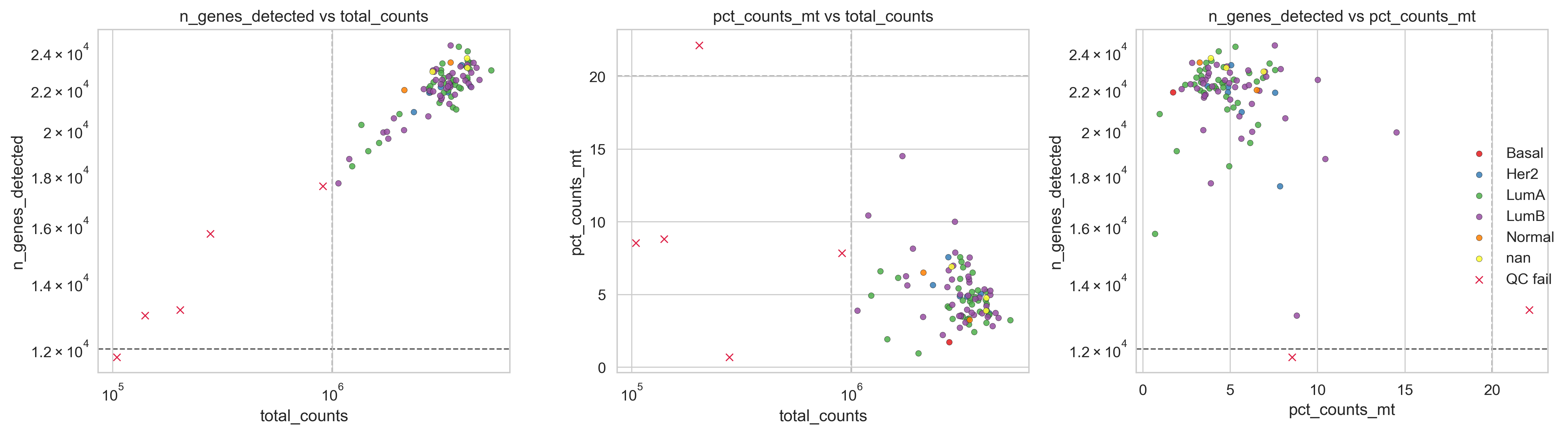
Example QC panel
What it does#
Creates a three-panel QC overview:
Genes vs total counts: library complexity vs sequencing depth.
Mitochondrial fraction vs total counts: mitochondrial contamination vs depth.
Genes vs mitochondrial fraction: gene complexity vs RNA integrity
All panels:
Use the same sample set
Share QC thresholds
Can be colored by a categorical variable (e.g. batch, subtype)
Optionally share a single legend for cleaner presentation.
This is intended as a one-stop QC diagnostic plot before filtering.
Requirements#
adata.obs must contain (by default):
total_counts_key → “total_counts”
n_genes_key → “n_genes_detected”
pct_mt_key → “pct_counts_mt”
Custom column names can be supplied via the *_key parameters.
Parameters#
Grouping#
groupby (str | None, default None). Optional categorical column in adata.obs used to color samples (e.g. “Batch”, “Subtype”).
QC thresholds#
Thresholds are applied consistently across all three panels.
min_counts / max_counts (float | None): Thresholds on total counts.
min_genes / max_genes (float | None): Thresholds on number of detected genes.
min_mt / max_mt (float | None): Thresholds on mitochondrial fraction (usually only max_mt is used).
Samples outside any specified threshold are marked as QC failures (internally handled by _scatter_qc).
Column keys#
total_counts_key (str, default “total_counts”).
Column in adata.obs for library size.
n_genes_key (str, default “n_genes_detected”).
Column in adata.obs for detected genes.
pct_mt_key (str, default “pct_counts_mt”).
Column in adata.obs for mitochondrial fraction.
Scaling#
log_counts (bool, default True).
Log-scale axes involving total counts.
log_genes (bool, default True).
Log-scale axes involving detected genes.
(Mitochondrial fraction is never log-scaled.).
Layout and output#
figsize (tuple[float, float], default (16.0, 4.6)).
Figure size in inches (wide by design).
share_legend (bool, default True). If True and groupby is provided, draws a single shared legend on the right instead of repeating it in each panel.
save (str | Path | None).
Path to save the figure.
show (bool, default True).
If True, calls plt.show().
Returns#
fig (matplotlib.figure.Figure). The figure object.
axes (np.ndarray[matplotlib.axes.Axes]). Array of the three subplot axes, in order:
genes vs counts
mt fraction vs counts
genes vs mt fraction.
Interpretation guide#
Panel 1 (genes vs counts).
Identifies low-complexity libraries and extreme depth outliers.
Panel 2 (mt% vs counts).
Highlights samples with high mitochondrial content regardless of depth.
Panel 3 (genes vs mt%).
Strong diagnostic for degraded or dying samples
(high mt%, low gene complexity).
Outliers that appear problematic in multiple panels are strong candidates for removal.
Examples#
Basic QC panel
bk.pl.qc_scatter_panel(adata)
Apply standard bulk RNA-seq thresholds
bk.pl.qc_scatter_panel(
    adata,
    min_counts=1e6,
    min_genes=12000,
    max_mt=8.0,
)
Color by batch with shared legend
bk.pl.qc_scatter_panel(
    adata,
    groupby="Batch",
    max_mt=7.5,
    share_legend=True,
)
Save without displaying
bk.pl.qc_scatter_panel(
    adata,
    max_mt=10.0,
    save="qc_panel.png",
    show=False,
)