PCA loadings bar plot#
- bullkpy.pl.pca_loadings_bar(adata, *, pc=1, n_top=15, loadings_key='PCs', use_abs=False, show_negative=True, gene_symbol_key=None, figsize=None, title=None, save=None, show=True)[source]#
Plot top PCA loadings for a single PC.
If use_abs=True: shows top |loading| (all positive bars).
Else: shows top positive and (optionally) top negative loadings.
Horizontal bar plot of the top PCA loadings for a single principal component (PC).
This is a compact, publication-friendly visualization to interpret which genes
drive a given PC, complementary to pca_loadings() (tables/GMT export).
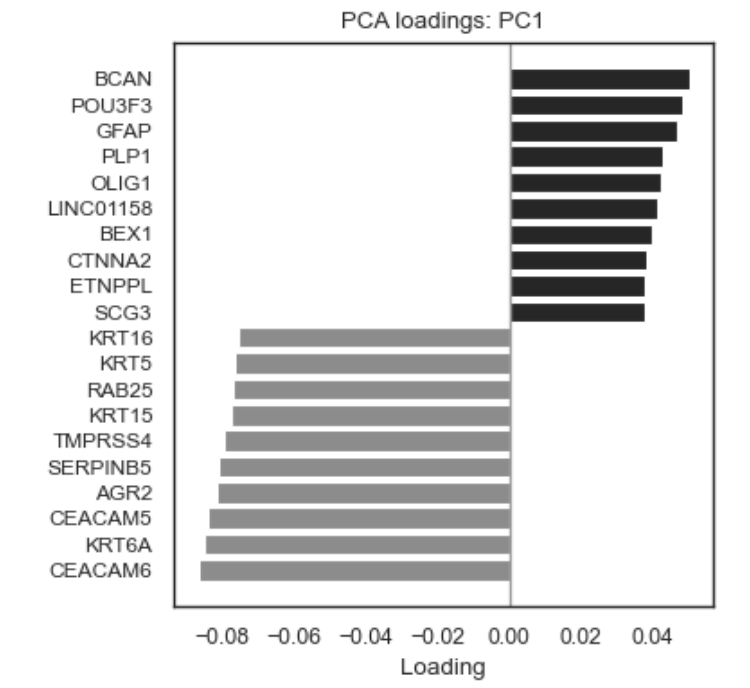
Example PCA loadings barplot
What it does#
Extracts PCA loadings from adata.varm[loadings_key]
Selects the strongest contributors for one PC
Plots them as a horizontal bar chart
Supports: – signed loadings (positive vs negative) – absolute loadings (magnitude only) – optional gene symbol mapping from adata.var.
Parameters#
Core inputs#
adata: AnnData.
Must contain PCA results:
adata.varm[loadings_key] → (n_genes × n_pcs) loadings matrix. Typically produced by bk.tl.pca().
pc: int, default 1.
Which principal component to plot (1-based indexing).
pc=1 → PC1
pc=2 → PC2.
n_top: int, default 15.
Number of top genes to show:
If use_abs=False: up to n_top positive and n_top negative genes
If use_abs=True: n_top genes by absolute loading
loadings_key: str, default “PCs”.
Key in adata.varm where PCA loadings are stored.
Ranking behavior#
use_abs: bool, default False.
False: – plot strongest positive loadings – optionally strongest negative loadings
True: – rank by |loading| – all bars plotted as magnitude-based contributors.
show_negative: bool, default True.
Only relevant when use_abs=False.
If False, shows only positive loadings.
Gene labeling.#
gene_symbol_key: str | None, default None.
Column in adata.var used for labels instead of adata.var_names.
(e.g. “gene_symbol” or “symbol”).
Fallback:
if not provided or missing → adata.var_names
Plot appearance#
figsize: tuple[float, float] | None. Auto-scaled by number of genes if None.
title: str | None.
Default: “PCA loadings: PC{pc}”.
Color convention:
Positive loadings → dark gray
Negative loadings → light gray
Absolute mode → neutral gray
Vertical reference line at x = 0
Output.#
save: str | Path | None.
If provided, saves the figure.
show: bool, default True.
Whether to call plt.show().
Returns#
(fig, ax)
fig: matplotlib.figure.Figure
ax: matplotlib.axes.Axes
Raises#
KeyError. If loadings_key not found in adata.varm.
ValueError.
If pc is outside the available PC range.
Examples#
Top signed loadings for PC1
bk.pl.pca_loadings_bar(
    adata,
    pc=1,
    n_top=15,
)
Only positive contributors for PC2
bk.pl.pca_loadings_bar(
    adata,
    pc=2,
    n_top=20,
    show_negative=False,
)
Absolute loadings (magnitude-only interpretation)
bk.pl.pca_loadings_bar(
    adata,
    pc=1,
    n_top=25,
    use_abs=True,
)
Use gene symbols instead of Ensembl IDs
bk.pl.pca_loadings_bar(
    adata,
    pc=3,
    gene_symbol_key="gene_symbol",
)
Save without displaying
bk.pl.pca_loadings_bar(
    adata,
    pc=1,
    save="PC1_loadings.png",
    show=False,
)
Notes & best practices#
Use signed mode (use_abs=False) to interpret directionality (opposing biological programs along a PC).
Use absolute mode (use_abs=True) to identify dominant drivers regardless of direction.
For enrichment analysis or exporting gene sets, prefer: – bk.tl.pca_loadings() (tables, GMT export).