Heatmap association#
- bullkpy.pl.heatmap_association(df, *, feature_col, groupby_col='groupby', value_col='effect', top_n=60, cmap='RdBu_r', center=0.0, figsize=None, title=None, save=None, show=True)[source]#
Heatmap of association values (effect by default), selecting top_n rows by best qval per column.
Heatmap visualization of association results across multiple groupings or contrasts.
This function summarizes association effect sizes (or any numeric value column) in a feature × contrast heatmap, allowing rapid comparison of patterns across multiple categorical association runs.
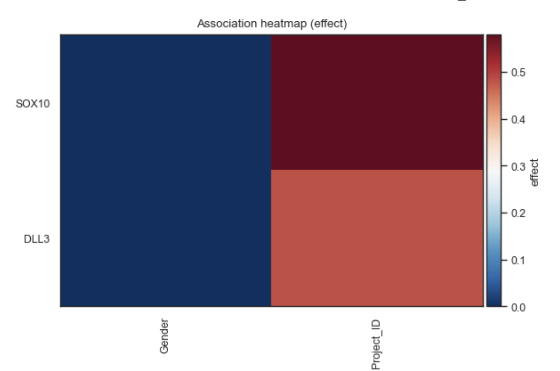
Example heatmap association plot
What it does#
Builds a wide matrix:
rows = features (genes or obs)
columns = groupby variables / contrasts
Displays values (default: effect size) as a heatmap
Automatically selects the top N features based on significance (q-value if available)
Uses a diverging colormap centered at zero (ideal for signed effects)
This plot is ideal for global pattern discovery and comparative summaries.
Expected input format#
A tidy pandas DataFrame containing:
column |
description |
|---|---|
feature_col |
gene or obs feature name |
groupby_col |
contrast / groupby identifier |
value_col |
numeric value to visualize (effect by default) |
qval (opt.) |
adjusted p-value used for feature ranking |
If qval is present, features are prioritized by significance.
Parameters#
df Association results table (long / tidy format).
feature_col
Column identifying features (genes or obs).
groupby_col
Column identifying contrasts or association runs.
value_col
Numeric column to display in the heatmap (default: “effect”).
top_n
Number of unique features to display.
cmap
Colormap used for the heatmap (default: “RdBu_r”).
center
Value at which to center the colormap (typically 0.0 for signed effects).
figsize
Figure size in inches. If None, determined automatically.
title
Optional plot title.
save
Path to save the figure.
show Whether to display the plot immediately.
Returns#
(fig, ax)
•	fig — matplotlib Figure
•	ax — matplotlib Axes
Examples#
Heatmap of gene associations across multiple contrasts
bk.pl.heatmap_association(
    df=assoc_df,
    feature_col="gene",
)
Visualize a different value column
bk.pl.heatmap_association(
    df=assoc_df,
    feature_col="gene",
    value_col="log2FC",
)
Limit to top 30 features
bk.pl.heatmap_association(
    df=assoc_df,
    feature_col="gene",
    top_n=30,
)
Save figure without displaying
bk.pl.heatmap_association(
    df=assoc_df,
    feature_col="gene",
    save="association_heatmap.png",
    show=False,
)
Interpretation guide#
•	Red cells → positive association (higher effect)
•	Blue cells → negative association (lower effect)
•	White / neutral → weak or near-zero association
Rows correspond to features; columns correspond to contrasts or groupby variables.
Notes#
•	Feature selection is global, not per contrast.
•	If qval is missing, feature order follows input order.
•	This function favors clarity and speed over clustering.
For hierarchical clustering or dendrograms, consider extending this plot.
See also#
•	pl.dotplot_association
•	pl.rankplot_association
•	pl.rankplot
•	pl.volcano
•	tl.gene_categorical_association
•	tl.obs_categorical_association